
DATA
Find the sources, dates, methods and limitations behind the Observatory’s maps and charts.
Briefings archive
Back to contentsRead current and past briefings with their original headlines, dates, sources and evidence. New editions do not overwrite published entries. Later source revisions are recorded separately. Briefings are prepared every two weeks when the evidence supports an update.
22 October 2026 · published edition
Atlantic · 22 Oct 2026 · El Niño shifts the Atlantic winter outlook.
Published 22 Oct 2026 · source checked 22 Oct 2026 · World Meteorological Organization; Met Office
El Niño is strengthening in the Pacific, with a peak forecast around December. WMO’s 21 October outlook favours above-average tropical Atlantic sea temperatures for November–January. The Met Office says El Niño can raise the likelihood of wetter, windier conditions in the UK during late autumn and early winter. These are seasonal probabilities, not predictions of individual storms; a quieter hurricane season does not mean a storm-free winter.
Seasonal outlook: November 2026–January 2027
Evidence and interpretation
- Analyse · what changed?
- This is a seasonal outlook, not a new Atlantic observation or fortnightly temperature average. WMO issued its November 2026–January 2027 outlook on 21 October, forecasting further El Niño strengthening towards a December peak and above-normal North and South Tropical Atlantic sea-surface temperatures. The UK weather context is from the Met Office’s 5 October explanation.
- Evaluate · how unusual is it?
- WMO reports close agreement among its forecast systems about El Niño strengthening; that is not a probability of a particular UK storm. The December peak is forecast, not an observed maximum. Baselines and regions differ across the source products, so no temperature-anomaly magnitudes are combined here. The Met Office describes shifts in likelihood, with other climate drivers also influencing the weather. No specific storm, cold spell, local flood or ecosystem impact is established by this outlook.
- Explain · what does it mean?
- El Niño develops in the tropical Pacific and can influence Atlantic weather through atmospheric circulation. Fewer tropical hurricanes and wetter, windier winter conditions elsewhere can coexist because hurricanes and winter weather systems are different. This outlook does not attribute our previously measured 40–45°N temperature patch or any individual weather event to El Niño. NOAA documented Isaias becoming a hurricane on 8 October UTC; the season is not hurricane-free.
Independent editorial summary of official seasonal forecasts and interpretation; no new forecast model or numerical anomaly calculation.
- Forecast peak and seasonal conditions may change.
- Seasonal probabilities cannot identify individual storms, landfalls or local impacts.
- Warm Atlantic water alone does not establish a marine heatwave or coral bleaching.
- Tropical Atlantic forecast conditions are separate from the fixed North Atlantic observation footprint.
Official outlook and interpretation pages checked 22 October. Forecast and interpretation sources rechecked for this edition. Forecast periods are separate from issue dates.
- Primary source
- WMO: Global Seasonal Climate Update for November–December–January · published 2026-10-21 · Forecast for November 2026–January 2027 · checked 22 Oct 2026.
- Met Office: El Niño and weather headline review · published 2026-10-05 · Late autumn and early winter seasonal context · checked 22 Oct 2026.
- NOAA: GOES East monitors Hurricane Isaias · published 2026-10-08 · 7 October CDT / 8 October UTC hurricane formation · checked 22 Oct 2026.
Independent summary of the linked official sources. No source images are reused.
Download this briefing and evidence · Archived calculation inputs
Arctic · 22 Oct 2026 · Autumn ice returns against a backdrop of long-term loss.
Published 22 Oct 2026 · source checked 22 Oct 2026 · NOAA/NSIDC Sea Ice Index, Version 4
Between 6 and 17 October, Arctic sea-ice extent grew by 758,000 km², but remained 19.7% below the 1981–2010 average for that date. Seasonal growth sits within a longer decline: NSIDC reports that 2007–2026 account for the 20 lowest annual summer minima in the satellite record. This hemisphere-wide comparison does not establish ice thickness or local wildlife impacts.
Observations: 1 October to 2026-10-17. Baseline: 1981–2010, same calendar day.
Evidence and interpretation
- Analyse · what changed?
- Arctic extent was 6.717 million km² on 2026-10-17, compared with 8.364 million km² for the same-calendar-day 1981–2010 reference. The difference is -1.647 million km², or -19.7%. The change since 6 October is +0.758 million km². The seasonal anomaly and the change over time are separate comparisons.
- Evaluate · how unusual is it?
- The reference uses 26 accepted years. The latest reading is within the descriptive mean ± two sample-standard-deviation band. Daily persistence and same-day historical comparisons are archived. This band is not a confidence interval, event probability or annual record. Daily values can be revised; zero missing coverage does not mean zero measurement uncertainty. Published context: The 20 years from 2007 to 2026 account for the 20 lowest annual Arctic minima in the satellite record. Its observation period is separate from this daily reading.
- Explain · what does it mean?
- Sea-ice extent describes hemisphere-wide coverage at the15% concentration threshold. Sea ice affects ocean–air exchange and habitat in general, but this hemisphere statistic alone cannot demonstrate local wildlife or community impacts. Thickness, ice duration, local exposure, causes and attribution are not established here.
Accepted same-calendar-day reference mean and sample SD(n−1); zero source Missing and nonnegative extent required.
- Daily provisional values may be revised. No measurement-error interval in this CSV. Zero Missing is not zero uncertainty.
- Mean ±2 sample SD is a descriptive reference band, not a confidence interval, event probability or attribution.
NSIDC product-page maintenance notice verified 22 October. Latest usable source dates rechecked 22 October; the provider file is unchanged.
- Primary source
- NSIDC: Arctic sea ice minimum ties for tenth lowest · published 2026-09-23 · Annual summer minima, 2007–2026 · checked 22 Oct 2026.
Sea Ice Index, Version 4 (Fetterer et al., 2025), DOI: 10.7265/a98x-0f50. Cite NSIDC; archived numerical subsets support these calculations.
Download this briefing and evidence · Archived calculation inputs
Antarctic · 22 Oct 2026 · Sea-ice extent nearly two million km² below the seasonal average.
Published 22 Oct 2026 · source checked 22 Oct 2026 · NOAA/NSIDC Sea Ice Index, Version 4
Antarctic sea-ice extent was 1.98 million km² below the 1981–2010 average for 16 October, a shortfall of 10.9%. All 16 accepted October readings lay below our descriptive historical comparison range. NASA reports that September’s winter maximum was the third lowest in the satellite record. These comparisons describe coverage; they do not establish local wildlife impacts. The newer, incomplete reading is excluded.
Observations: 1 October to 2026-10-16. Baseline: 1981–2010, same calendar day.
Evidence and interpretation
- Analyse · what changed?
- Antarctic extent was 16.225 million km² on 2026-10-16, compared with 18.200 million km² for the same-calendar-day 1981–2010 reference. The difference is -1.975 million km², or -10.9%. The change since 6 October is -0.481 million km². The seasonal anomaly and the change over time are separate comparisons.
- Evaluate · how unusual is it?
- The reference uses 28 accepted years. The latest reading is below the descriptive mean ± two sample-standard-deviation band. Daily persistence and same-day historical comparisons are archived. This band is not a confidence interval, event probability or annual record. Daily values can be revised; zero missing coverage does not mean zero measurement uncertainty. Published context: The annual maximum reached 17.59 million km² on 14 September, third lowest in the satellite record. Its observation period is separate from this daily reading.
- Explain · what does it mean?
- Sea-ice extent describes hemisphere-wide coverage at the15% concentration threshold. Sea ice affects ocean–air exchange and habitat in general, but this hemisphere statistic alone cannot demonstrate local wildlife or community impacts. Thickness, ice duration, local exposure, causes and attribution are not established here.
Accepted same-calendar-day reference mean and sample SD(n−1); zero source Missing and nonnegative extent required.
- Daily provisional values may be revised. No measurement-error interval in this CSV. Zero Missing is not zero uncertainty.
- Mean ±2 sample SD is a descriptive reference band, not a confidence interval, event probability or attribution.
NSIDC product-page maintenance notice verified 22 October. Latest usable source dates rechecked 22 October; the provider file is unchanged. The Antarctic 17 October row has 0.382 million km² of missing coverage and is excluded.
- Primary source
- NASA: Antarctic Sea Ice Grows to Its 2026 Maximum · published 2026-10-12 · 2026-09-14 annual maximum · checked 22 Oct 2026.
Sea Ice Index, Version 4 (Fetterer et al., 2025), DOI: 10.7265/a98x-0f50. Cite NSIDC; archived numerical subsets support these calculations.
Download this briefing and evidence · Archived calculation inputs
Greenland · 22 Oct 2026 · Robots measure melting at Greenland’s glacier face.
Published 22 Oct 2026 · source checked 22 Oct 2026 · British Antarctic Survey · GIANT expedition
During summer 2026, a BAS-led team aboard RRS Sir David Attenborough studied Sorgenfri Gletsjer and its fjord in East Greenland. A sensor placed in the glacier face collected measurements for 19 hours, alongside surveys by underwater robots. Researchers will use the observations to improve models of glacier melting and freshwater movement into the Atlantic. BAS reported the expedition on 9 October; the report does not give a new ice-sheet-wide melt estimate.
Fieldwork: summer 2026 · Expedition report: 9 October 2026
Evidence and interpretation
- Analyse · what changed?
- BAS’s 9 October expedition report describes summer 2026 fieldwork at Sorgenfri Gletsjer in East Greenland. The team worked in the fjord for 30 days, deployed instruments 523 times and obtained 19 continuous hours of Meltstake measurements close to the glacier face. These are expedition achievements and measurement duration, not a quantified regional melt rate or a fortnightly change.
- Evaluate · how unusual is it?
- This is an official expedition report, not a peer-reviewed analysis of the resulting measurements. BAS describes the first Meltstake deployment in Greenland; the briefing does not extend that claim to all glacier research. The report does not specify exact fieldwork dates, a new whole-ice-sheet mass-loss estimate, a historical melt ranking, or uncertainty bounds on a melt-rate result. Photos have named credits and are not reused here.
- Explain · what does it mean?
- Researchers intend to improve understanding and models of glacier–ocean melting, fjord mixing and freshwater transport into the North Atlantic. These are research aims, not proof that a circulation tipping point has occurred or a prediction of its date. BAS says analysis and model development will continue over the following three years. The annual mass-balance briefing remains a separate dated record; a small source revision checked 22 October is noted beside the archive.
Independent editorial summary of the official BAS expedition report; no new ice-loss calculation.
- Fieldwork occurred during summer, not this fortnight.
- The report describes data collection and planned analysis, not a new whole-ice-sheet melt estimate.
- No circulation tipping point or local ecosystem impact is demonstrated by the report.
- Nineteen hours is sensor measurement duration, not the length of the expedition.
BAS report checked 22 October. Exact fieldwork dates are not stated in this report. The previous annual mass-balance briefing remains dated 8 October in the archive.
- Primary source
- BAS: Robot fleet studies Greenland’s melting glaciers · published 2026-10-09 · Summer 2026; 30 days in an East Greenland fjord · checked 22 Oct 2026.
Independent summary of the linked official sources. No source images are reused.
Download this briefing and evidence · Archived calculation inputs
8 October 2026 · published edition
Atlantic · 8 Oct 2026 · A warm patch persists in the North Atlantic.
Published · data through 6 Oct 2026 · NOAA OISST v2.1
Across a patch covering around 350,000 km², average surface temperatures stayed at least 2°C warmer than its seasonal average in the five daily analyses from 2–6 October. This is a persistent surface pattern, but its historical rarity and effects on marine life have not been assessed. It is not yet classified as a marine heatwave.
Evidence and interpretation
- Analyse · what changed?
- Ocean-surface temperature averaged +3.41 °C above the NOAA 1971–2000 seasonal baseline across a 353,654 km² footprint on 6 October 2026.
- Evaluate · how unusual is it?
- The accepted tiles stayed at least +2 °C above baseline in five consecutive daily analyses. Common valid coverage was 100%. Historical percentiles, formal heatwave criteria and an analysis-error assessment were unavailable; the older baseline should not be read as today’s climate normal.
- Explain · what does it mean?
- The reading identifies a sustained surface-temperature pattern worth following. Local ecosystem effects and causes have not been assessed. No claim of harm or climate attribution is made.
Largest absolute patch-mean anomaly among candidates covering at least 100,000 km². Selection is a screening heuristic, not a historical rarity score.
Derived patch mean: +3.41 °C on 6 Oct 2026. Area: approximately 353,654 km², across 39 adjoining 1° tiles. This is an irregular footprint within 60–45°W and 40–45°N, not the entire bounding rectangle.
| Analysis date | Difference (°C) |
|---|---|
| 2 Oct 2026 | +2.92 |
| 3 Oct 2026 | +3.09 |
| 4 Oct 2026 | +3.29 |
| 5 Oct 2026 | +3.29 |
| 6 Oct 2026 | +3.41 |
Screening used six named Atlantic search windows. The map outline follows the 1° screening tiles, not a measured ocean front. Each accepted 1° tile had a mean anomaly of at least +2 °C on all five consecutive days, with at least 90% common valid coverage. Patch means are weighted by grid-cell area. The source is preliminary; no historical percentile or analysis-error test was available.
- Named search windows only; not a basin-wide search.
- Threshold is an editorial screening choice, not a percentile or heatwave definition.
- Persistence is limited to five saved daily analyses; earlier onset is unknown.
- Source analyses may be preliminary and are not independent station observations.
- No per-cell analysis error or historical daily percentile is present in this saved feed.
- Areas use spherical grid-cell geometry; source ice >=15% and missing/invalid SST or anomaly are excluded.
- Missing ice fraction is not zero. Such cells are screened only when SST is at least 5 C on every day; this omits colder-water candidates and does not verify absence of ice.
- Components stop at search-window boundaries.
Source and dataset · Map methods · Download this briefing and evidence · Archived calculation inputs
The evidence file freezes the values, source dates, selection method, limitations and source-file checksums for this briefing. Later map updates do not rewrite this entry.
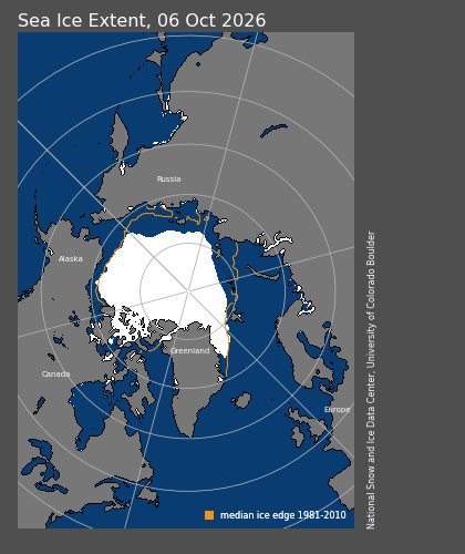
Arctic · 8 Oct 2026 · Arctic sea ice is below its seasonal average.
Published · data through 6 Oct 2026 · NOAA/NSIDC Sea Ice Index, Version 4
Sea ice covered 5.959 million km² on 6 Oct 2026. The reading is still within the historical comparison range used here. Extent describes the area covered by sea ice. This daily comparison helps track the seasonal ice cover; it does not establish changes in thickness, wildlife impacts or a long-term trend.
Evidence and interpretation
- Analyse · what changed?
- Arctic sea-ice extent was 5.959 million km² on 6 October 2026, 19.3% below the same-calendar-day 1981–2010 reference mean.
- Evaluate · how unusual is it?
- The central estimate remains inside the descriptive reference range, mean plus/minus two sample standard deviations. This uses 28 valid reference years. The range is not a confidence interval; no source uncertainty interval is available in this saved daily record, and recent values may be revised.
- Explain · what does it mean?
- This tracks seasonal sea-ice coverage. It does not measure thickness or land-ice loss; wildlife effects and a long-term trend cannot be established from this daily comparison.
First editorial example: latest saved hemisphere-wide extent and its existing same-calendar-day comparison.
Extent: 5.959 million km². Same-day reference mean: 7.388 million km². Difference: -19.34%. Reference range: 5.282–9.495 million km²; the reading is within this range.
The reference uses 28 valid years from 1981–2010 for the same calendar day. The range is the mean plus or minus two sample standard deviations.
- One daily reading does not establish a long-term trend or a record minimum.
- Mean ± two sample standard deviations describes the reference period; it is not a probability or confidence interval.
- Extent is a satellite-derived estimate at the 15% concentration threshold, separate from the OSI SAF map product.
- Recent daily values may be revised.
View the cited 6 Oct 2026 sea-ice map · Provider daily record
Source and dataset · Map methods · Download this briefing and evidence · Archived calculation inputs
The evidence file freezes the values, source dates, selection method, limitations and source-file checksums for this briefing. Later map updates do not rewrite this entry.
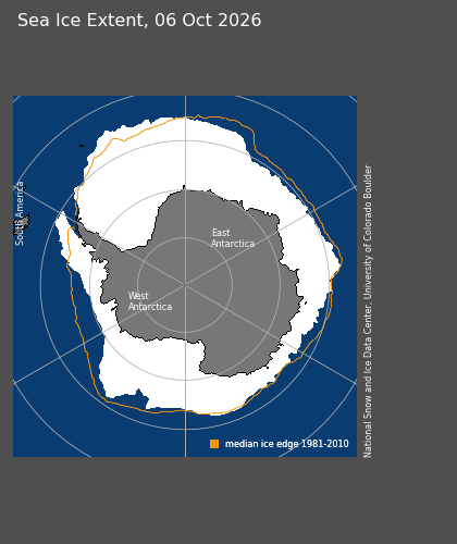
Antarctic · 8 Oct 2026 · Antarctic sea ice is below its seasonal average.
Published · data through 6 Oct 2026 · NOAA/NSIDC Sea Ice Index, Version 4
Sea ice covered 16.706 million km² on 6 Oct 2026. That puts it below the historical comparison range used here. Extent describes the area covered by sea ice. This daily comparison helps track the seasonal ice cover; it does not establish changes in thickness, wildlife impacts or a long-term trend.
Evidence and interpretation
- Analyse · what changed?
- Antarctic sea-ice extent was 16.706 million km² on 6 October 2026, 9.4% below the same-calendar-day 1981–2010 mean.
- Evaluate · how unusual is it?
- The central estimate is below the descriptive mean plus/minus two sample-standard-deviation range based on 28 valid years. This is not a record-low or probability claim. No source uncertainty interval is available in the saved daily record; recent values may be revised.
- Explain · what does it mean?
- The comparison identifies reduced seasonal sea-ice coverage relative to the reference period. It does not establish ice thickness, wildlife impacts or a long-term trend, and it is separate from land-ice loss.
First editorial example: latest saved hemisphere-wide extent and its existing same-calendar-day comparison.
Extent: 16.706 million km². Same-day reference mean: 18.443 million km². Difference: -9.42%. Reference range: 17.675–19.211 million km²; the reading is below this range.
The reference uses 28 valid years from 1981–2010 for the same calendar day. The range is the mean plus or minus two sample standard deviations.
- One daily reading does not establish a long-term trend or a record minimum.
- Mean ± two sample standard deviations describes the reference period; it is not a probability or confidence interval.
- Extent is a satellite-derived estimate at the 15% concentration threshold, separate from the OSI SAF map product.
- Recent daily values may be revised.
View the cited 6 Oct 2026 sea-ice map · Provider daily record
Source and dataset · Map methods · Download this briefing and evidence · Archived calculation inputs
The evidence file freezes the values, source dates, selection method, limitations and source-file checksums for this briefing. Later map updates do not rewrite this entry.
Greenland · 8 Oct 2026 · Greenland lost ice over the latest annual period.
Published · data through 31 Aug 2026 · PROMICE mass balance product (Mankoff et al. 2021)
Greenland’s ice sheet lost an estimated 191 billion tonnes over September 2025–August 2026. This is the balance between ice gained and ice lost across the whole ice sheet. The estimate lies within the 1990/91–2019/20 historical range, with source uncertainty of ±98 billion tonnes. It records a net reduction in land ice, which contributes to sea-level rise; it does not describe the past fortnight.
Evidence and interpretation
- Analyse · what changed?
- The saved PROMICE record estimates net whole-ice-sheet balance of −191.147 Gt over 1 September 2025–31 August 2026.
- Evaluate · how unusual is it?
- The central estimate lies within the mean plus/minus two sample-standard-deviation range of the 30 annual balances from 1990/91–2019/20 (-442.2 to 127.3 Gt). Source uncertainty is ±98.317 Gt; no unsupported confidence level is assigned. Within the range does not imply a stable ice sheet.
- Explain · what does it mean?
- Net loss of land ice contributes to sea-level rise. This is an annual balance estimate rather than local melt or glacier speed; we have not calculated a sea-level contribution from this value.
Latest complete annual estimate in the saved PROMICE record. This is an annual context briefing, not a newly detected fortnightly anomaly.
Annual net mass balance: -191.147 Gt; source uncertainty ±98.317 Gt. Period: 1 September 2025–31 August 2026. Retrieved 4 Oct 2026. One Gt is one billion tonnes.
Estimate from surface-mass-balance models, solid-ice discharge and basal mass balance. PROMICE / Mankoff et al. (2021), CC BY 4.0. This briefing rounds the source values; no claim of statistical significance or record loss is made.
- Annual estimates may be revised.
- Source uncertainty is preserved without assigning an unsupported confidence level.
- Ice mass balance is distinct from glacier surface speed and sea-ice extent.
Provider annual record · NASA · land ice and sea level · CC BY 4.0
Source and dataset · Map methods · Download this briefing and evidence · Archived calculation inputs
The evidence file freezes the values, source dates, selection method, limitations and source-file checksums for this briefing. Later map updates do not rewrite this entry.
Greenland annual estimate · source revision checked 22 Oct 2026
The 8 October briefing above preserves its published estimate of 191 ±98 billion tonnes of net ice loss for September 2025–August 2026. The GEUS/PROMICE annual source checked on 22 October revises that same period to 192 ±98 billion tonnes (net balance −192.291 Gt; supplied uncertainty ±98.412 Gt). This is a revision to an annual estimate, not an additional 1.14 billion tonnes lost since the briefing.
Saved original and revised source records · Provider annual record. PROMICE / Mankoff et al. (2021), CC BY 4.0. No confidence level is added to the supplied uncertainty.
Global globe
Back to contentsSources, dates and reuse terms for the Global globe. These are dated snapshots, with no automatic updates configured. Human activity alone does not establish environmental harm. Missing coverage is not evidence of absence.
Explore · reference geography, seabed names and major reefs
Explore opens a plain reference globe. Coastal names become more detailed as you zoom; named seabed features use representative label markers. Coastal names, seabed names and reef outlines can be switched independently. This is a geographic atlas, not a navigation chart.
Seabed names: IHO-IOC GEBCO Gazetteer of Undersea Feature Names, www.gebco.net, distributed by NOAA NCEI / IHO DCDB. Saved 18 October 2026 from all three official point, line and polygon layers: 5,310 distinct named features after combining repeated feature IDs and omitting one unknown-type record. Generic types include banks, shoals, canyons, ridges, trenches and channels. AO uses the spherical mean of each feature’s source geometry vertices as a representative label position; markers are not surveyed hazard positions or feature boundaries. Feature coordinates shown are rounded label anchors, not a statement of positional accuracy. The red pointer marks a location selected on the reference globe; its coordinates are not a surveyed depth or hazard position. Find location and shared Explore links can retain this pointer.
Coastal names and major reefs: Natural Earth reference geography. Existing ocean, sea, gulf, bay, strait, sound, channel, fjord, island and cape labels are retained. Major reef outlines are from Natural Earth’s 1:10m reefs distribution (version 4.0.0), derived from WDB2. These are generalised, incomplete reference outlines; Natural Earth documents poor definition in some areas, including the Great Barrier Reef. They do not show current reef condition, water depth or safe passage. Natural Earth data are public domain.
Names are selected by zoom, available space and proximity to the visible hemisphere. A missing label or outline does not imply that a feature is absent. Banks and shoals here are named geographic features, not a complete inventory of underwater hazards. Buoys, lights, wrecks, obstructions, surveyed depths, tides and safe shipping routes are not supplied. Use appropriate current official charts for navigation.
The saved date records retrieval, not an observation, survey or legal effective date. Source versions, scope, adaptation methods and checksums · Reef source and known limitations ↗ · Open Explore ↗.
Ocean climate · coral heat stress
NOAA Coral Reef Watch v3.1 Degree Heating Week (DHW), provided through NOAA CoastWatch ERDDAP. Native 0.05° grid (about 5 km); daily satellite-derived product. The globe shows the latest verified field, 20 October 2026, with a source reference time of 12:00 UTC. This is a daily date marker, not a claim that every satellite observation occurred at noon. Checked 22 October 2026: the primary NOAA STAR archive and CoastWatch mirror both reach 20 October. A source publication date and retrieval/check time are separate. This layer is a saved snapshot; an automatic production refresh is not yet configured.
DHW combines the intensity and duration of thermal exposure over the preceding 84 days, in °C-weeks. NOAA accumulates daily Coral Bleaching HotSpot values of at least 1 °C above its Maximum Monthly Mean reference, divided by seven. The threshold climatology represents 1985–1990 plus 1993, derived from a longer record and recentered by NOAA. It is different from our OISST temperature-anomaly baseline; the two fields must not be subtracted or interpreted as interchangeable. AO uses the supplied DHW field rather than calculating a new index from OISST.
The numerical snapshot retains every valid native grid value in hundredths, split into four lossless tiles. Land, ice, missing values and values masked by the provider’s declared 0–100 valid range remain unavailable; they are never replaced with a nearby ocean value or clipped into validity. The manifest records excluded water values separately. Selecting the globe reads the nearest native grid cell. Zoom does not add source resolution.
The globe colour overview uses the maximum available native value within each 0.1° display cell (2 × 2 native cells). Devices with smaller texture limits use 0.2° or 0.4° blocks with the same maximum rule. These maxima preserve higher local exposure in the broad overview; they do not change numerical point readings. The selected point can therefore differ from its surrounding overview colour. Entirely missing blocks remain missing. The colour scale saturates at 20 °C-weeks; point readings retain valid higher values.
Heat stress can indicate potential coral bleaching risk. This is not observed bleaching, a mortality estimate, a forecast or an overall ocean-health score. The global numerical field includes ocean cells without coral reefs; an offshore colour does not establish a local coral impact. DHW alone does not determine NOAA’s Bleaching Alert Area category, which also depends on HotSpot and a defined time window. We do not infer those alert categories from DHW. NOAA’s current alert scheme includes Levels 1–5; older mirror category metadata must not truncate it.
Major reef outlines reuse the Natural Earth public-domain reference geography already used by Explore. They are generalised and incomplete, become visible on closer views, and carry no current reef-condition information. Source and coastline masks can differ around small islands. This view does not resolve reef-depth temperatures, local shading, species sensitivity, acclimatisation or other causes of ecological variation.
NOAA product methods ↗ · Numeric data service ↗ · Dataset citation ↗ · Saved date, coverage and checksums. Credit: NOAA Coral Reef Watch. Current CRW products are freely reusable with attribution; NOAA does not endorse this adaptation. Reuse and citation guidance ↗.
Ocean Climate · daily sea-surface temperature and anomaly
NOAA/NCEI Optimum Interpolation Sea Surface Temperature (OISST) v2.1. Daily analysed surface fields on the native global 0.25° grid. This layer uses the preliminary 13 October 2026 analysis, retrieved 15 October 2026. The globe displays the source analysis date, not the retrieval date; noon UTC in the source identifies the daily field, not the time every observation was made. This is a saved snapshot; automatic updates have not yet been configured.
Temperature is sea-surface temperature in °C, separate from air temperature and the heat stored through the water column. Anomaly uses NOAA’s supplied difference from its 1971–2000 daily seasonal climatology, without rebasing or calculating a new anomaly. Blue is cooler, red warmer and zero is neutral. An older baseline is not today’s climate normal. A warm anomaly alone does not establish a marine heatwave, ecological harm or its cause.
The numerical fields share one mask: source land/missing SST or anomaly, and cells with a known NOAA ice-proxy fraction of at least 15%, are excluded from both views. The NOAA ice field helps its SST analysis estimate temperatures near ice; it is not AO’s independent sea-ice concentration layer. Missing ice-proxy values are retained as missing, not changed to zero; otherwise valid SST and anomaly remain available. Grey ocean has no displayed reading and should not be interpreted as cold water or verified absence of ice. Coastline geography can differ from the analysis grid.
AO preserves all native grid-cell values and rotates the longitude ordering into −180° to 180° for display. Tapping a location reads the containing native grid cell; it does not move to a nearby valid cell or interpolate a new value. Display readings round to 0.1 °C. Temperature colours saturate at −2 and 35 °C; anomaly colours at −5 and +5 °C. Readings retain source values beyond these colour limits. Land and ice-masked waters remain excluded while changing views.
NOAA combines satellite, ship and buoy observations into a spatially complete analysis over its valid ocean domain. This is a grid estimate, not a thermometer measurement at the selected point. Preliminary fields may be revised. The source includes an SST analysis-error field; this first global view does not display uncertainty or infer anomaly confidence. It is not intended for navigation or operational decisions.
NOAA product and methods ↗ · Dataset citation ↗ · Source daily NetCDF ↗ · Saved field dates and checksums · Snapshot provenance. NOAA data are publicly available; NOAA does not endorse this adaptation.
Ocean climate · global surface currents
FNMOC ESPC-D V02 / HYCOM, distributed by HYCOM.org. The dated saved field uses forecast hour zero, valid at the displayed model run time. The map and saved manifest show the run and valid times; retrieval and the latest refresh check are separate records. These are instantaneous model velocities at 0 m, not daily means, direct measurements or a map of the deep overturning circulation. The model metadata describe its operational status as pre-operational. A daily scheduled source check publishes only validated paired fields. It verifies units, coordinates, depth, time, mask pairing and coverage; rejects older, future or over-72-hour-old source runs; and keeps the previous manifest and field if retrieval or validation fails. Fixed source metadata are checked for revisions before reusing an unchanged run. The refresh-status record exposes success or retained data without changing the scientific timestamp. Fields older than 72 hours are labelled as older saved data on the map.
AO takes every tenth longitude and twentieth latitude from the provider’s regular 0.08° × 0.04° delivery grid, producing a 0.8° display sample. The saved vectors are not averaged or interpolated. Display streamlines use the separate interpolation described below. The delivered grid covers 80°S to 90°N; retained latitude centres end at 89.6°N. The source model’s native grid is finer than this delivery and preview. Land and missing vectors stay missing. Display geography and model coastlines can differ, especially near islands and narrow channels.
Curved streamlines illustrate the instantaneous surface-flow pattern, with arrowheads towards the flow. AO traces short paths through the frozen field in both directions using a spherical midpoint method at 0.2° spatial steps, with bilinear interpolation only where all four surrounding retained grid points are valid. Tracing stops at missing data, weak flow below 0.01 m/s, the coverage limits or 85° latitude; completed small loops are not repeatedly traced. Paths are display samples, not measured tracks or predictions. Traced lines are projected onto the globe and drawn as local quadratic Bezier curves; these short control segments avoid the overshoot of long decorative handles. Lines thin with zoom and screen spacing. Line colour represents local interpolated speed from 0 to 2 m/s, saturating at 2 m/s. Arrowheads show direction; line length and spacing do not represent speed, volume or elapsed time. Gaps can reflect display thinning, weak flow or missing coverage.
Tapping still reads the nearest retained model grid point without interpolating its numerical value or substituting another ocean point. Speed is √(u²+v²); bearing is clockwise from true north, towards the flow. Readings retain speeds above the colour limit. These are instantaneous streamlines, not time-evolving particle trajectories.
The model assimilates observations and is driven by atmospheric forcing. This view does not display uncertainty or separately identify tidal and wave-driven drift components, and is not for navigation. It cannot establish the present movement of plastic: the separately labelled accumulation zones represent a historical modelling study with different dates and methods.
Official product, grid and model documentation ↗ · Public source catalogue ↗ · Saved run, valid time and checksum · Latest refresh check. Source metadata permit public release with unlimited distribution; the catalogue labels the data freely available. Credit: FNMOC / HYCOM.org. No endorsement is implied.
Historical shipping · January 2015–February 2021
World Bank / IMF World Seaborne Trade Monitoring System (Cerdeiro, Komaromi, Liu and Saeed, 2020). Commercial-vessel AIS position reports accumulated from January 2015 to February 2021, including moving and stationary ships. Retrieved 13 October 2026. This is historical reporting activity, not current routes, vessel counts or measured environmental impact.
AO summed the source grid into a smaller display raster and applied a logarithmic colour and opacity scale. One worldwide scale runs from lighter teal (#7bc8c5) through pale green (#9bcdb4), cream (#efd792) and peach (#e28b60) to red (#b0394e) as recorded activity increases. Cream is a colour transition, not an average or normal baseline. The stored intensity follows a squared logarithmic scale, capped at the 99th percentile of positive cells. A smooth, increasing display curve softens the middle tones so busier corridors stand out; the faintest readings retain their opacity. This styling does not change the source counts or their ordering. There is no lower-percentile cutoff; very small readings remain faint, and the top 1% shares maximum colour and opacity. Angular cells have unequal physical areas, so this is relative activity, not density per square kilometre. Coverage stops near 85° north and south. Blank areas can reflect no reports, weak displayed activity or unavailable coverage.
Shipping shading is clipped to water in the Natural Earth reference map; the underlying activity raster is unchanged. Coastal water and estuaries remain visible where the map resolves them. Narrow rivers and most inland waters are not represented by this land mask, so this view is not a complete inland-waterway map. Clipping removes inland marks from view; it does not validate the remaining AIS reports.
Port names and reference points come from Natural Earth’s 1:10m ports, version 5.0.0 (1,081 records; retrieved 21 October 2026). More names appear as you zoom, using the source’s cartographic scale ranks and spacing to avoid overlapping labels. These ranks do not measure traffic. Locations may be approximate and names historical; this is not a complete current port inventory or a navigation chart. Port markers do not connect individual AIS reports to ports or show live arrivals.
Natural Earth port source and location limitations ↗ · Public-domain terms ↗ · Port layer provenance and checksum.
World Bank source and methods ↗ · CC BY 4.0 licence ↗. AO’s aggregation and display styling are adaptations of the source raster.
Offshore wind · February 2026 inventory
Global Wind Power Tracker, Global Energy Monitor, February 2026 release. Retrieved from GEM’s public map data on 13 October 2026. The globe includes 2,085 offshore project-phase locations across 57 countries and areas. A point represents a project phase, not an individual turbine; a farm can have several phases.
GEM principally tracks phases above 10 MW, with some smaller projects included. Coverage is incomplete and most locations in this subset are approximate. Operating, construction, announced, pre-construction, shelved, cancelled and retired records remain distinct. The release date is not a common observation date or a current operational check; project facts have different dates. A start year may be actual or planned, depending on status. Capacity, where given, is phase nameplate capacity rather than measured generation or environmental impact.
The source’s exact/approximate location flag is retained. “Exact” is the provider’s classification, not an AO survey or a legal boundary. Country and area labels follow the publisher’s economic contexts rather than strict political boundaries. This subset comes from GEM’s separately published public map data; its totals can differ from tracker headline figures. Shared locations and legitimate phases are retained.
AO selected offshore installation types, retained source status and location-accuracy fields, normalized the records and rounded coordinates to six decimals. © Global Energy Monitor. Tracker, methods and citation ↗ · GEM reuse terms ↗ · CC BY 4.0 licence ↗.
Microplastics · samples & accumulation zones
Worldwide plastic accumulation zones
Pink hatching shows five historical modelled accumulation cores in the North Pacific, North Atlantic, South Pacific, South Atlantic and Indian Ocean subtropical gyres. The North Pacific contour represents accumulation in the gyre associated with the Great Pacific Garbage Patch; it does not reproduce the separate 2018 study boundary. These are illustrative research contours, not current patch boundaries, floating islands, a complete pollution inventory or measurements of today's conditions. Unmarked water can contain plastic. Equal hatching does not imply equal concentrations or equal total amounts between zones.
Source: Eriksen et al. (2014), using surveys from 2007–2013 and a calibrated ocean-dispersal model. The numerical model rasters were deposited by Laurent Lebreton in 2021, and retrieved for this layer on 21 October 2026. The deposit and retrieval dates are not observation dates. The separate NOAA NCEI sample archive retains its own sampling dates and methods below.
Derivation by Atlantic Observatory: convert each published log10 count-density raster to particle counts, sum the two microplastic size classes (0.33–1 mm and 1.01–4.75 mm), and retain the largest contiguous model area at or above 50,000 particles/km² within each subtropical gyre. Basin windows identify components without cutting their outlines. Simplify contours by 0.15° while preserving topology and split at the date line. This display threshold was chosen by the Observatory to identify accumulation cores; it is not an author-issued garbage-patch definition, ecological risk threshold or alert. The broader accumulation regions extend beyond the outlines and move with ocean conditions.
The historical model uses particles/km² at the surface. Selected water samples use particles/m³; these are different quantities and cannot be compared directly. Sample-year filters apply only to the points, not to the historical hatching. Visibility controls allow either evidence layer to be hidden. The hatching is clipped to the globe's reference ocean mask.
Eriksen et al. 2014 · original research ↗ · Lebreton · published model rasters ↗ · CC BY 4.0 · Download derived contours, provenance and method.
Nyadjro, Ebenezer; Webster, Jennifer; Boyer, Tim; Cebrian, Just; Collazo, Leonard; Kaltenberger, Gunnar; Larsen, Kirsten; Lau, Yee; Mickle, Paul; Toft, Tiffany; Wang, Zhankun (2025). The NOAA NCEI Global Marine Microplastics Harmonized Database during 1972-04-20 to present, NCEI Accession 0306475. NOAA National Centers for Environmental Information. AO’s subset contains 16,988 ocean-water measurements in particles per cubic metre, collected from 20 April 1972 to 23 October 2024. Accessed 13 October 2026. The default selection is 2020–2024. NOAA updates its archive quarterly; this view is a saved snapshot.
AO selected valid dated ocean-water records in the same units, retaining zero readings, sampling method, mesh size, depth and original-study links. Beach and sediment samples are excluded. No interpolation, averaging, unit conversion or concentration classification is added. Globe readings use up to three significant digits for readability, with ≈ marking rounded values; selected records on this page retain the supplied precision. Equal pink dots mark samples; outlined groups collect nearby samples for readability. Size and colour do not encode concentration.
Sampling is uneven. A gap does not mean clean water, and a zero result does not show that surrounding water is plastic-free. Methods, depths and mesh sizes differ; matching units alone do not make studies directly comparable. Select a sample to open its original study and read its methods.
Dataset citation ↗ · NOAA metadata and reuse terms ↗ · Methods and limitations ↗ · CC0 1.0 public-domain dedication ↗. Source links and credits are retained; NOAA does not endorse this adaptation.
The globe’s coastlines, borders and labels use Natural Earth public-domain geography. AO adapts their display to the globe. The reference blue ocean and grain are decorative. Ocean climate shows temperature fields or surface-current vectors only when selected. Red story markers identify approximate regions, not precise study stations or complete study areas; follow each story for its actual place and observation period. Layer licences apply separately; there is no single licence for every photograph, dataset or other resource on this site.
Atlantic maps
Back to contentsSources and methods for each Atlantic map layer.
Sea-surface temperature and anomaly
NOAA/NCEI OISST v2.1, supplied via NOAA CoastWatch ERDDAP. ANALYSIS · °C · native 0.25° grid · daily surface fields. Atlantic map coverage is 65°S–75°N, 85°W–25°E. Preliminary values can be revised. Saved daily dates appear in the map time controls.
SST anomaly is the difference from NOAA’s 1971–2000 daily climatology. Positive values are warmer; negative values are cooler. Colours saturate at the legend endpoints; point readings retain the actual value. Temperature and anomaly use different scales.
Daily air temperature and anomaly
The air toggle uses Copernicus Climate Change Service / ECMWF ERA5 reanalysis at 2 metres above land, ocean and sea ice. It is a grid-cell estimate combining observations and modelling, not a local thermometer reading. The map displays its own valid UTC day. A separate daily updater retrieves saved public fields directly from the Copernicus Climate Data Store; page loading does not start a download.
Temperature is the average of all 24 hourly records in a UTC day. The anomaly subtracts the average for the same calendar day over 1991–2020, using the same ERA5 variable and grid. The Copernicus daily statistics service averages hourly records and removes partial periods. The historical normal requires all 30 requested yearly daily fields; the updater checks their dates, grid and coverage before publication. February 29 uses the mean of the February 28 and March 1 normals.
The regular 0.25° source grid is sampled every 0.5° for display. Colour shading blends adjacent valid grid-node colours. Point readings use the nearest sampled source node; missing data is not filled. Screen shading and zoom do not add scientific resolution. Missing data remains unavailable. Blue denotes cooler and red warmer than the historical mean. Anomaly colours stop at ±10 °C; numeric readings retain the actual value. No separate anomaly uncertainty is supplied.
Reanalysis arrives after a delay; recent ERA5 values may be preliminary and revised. The air map keeps its own date, which can differ from the ocean and ice layers. A single daily anomaly does not establish a long-term trend. Forecasting is not included in this air comparison.
Contains modified Copernicus Climate Change Service information (2026). Official ERA5 source, DOI and licence ↗ · Copernicus daily statistics, DOI and CC-BY 4.0 licence ↗. Contains modified Copernicus Climate Change Service information. The European Commission and ECMWF are not responsible for use of this information. Daily source processing retains the previous snapshot if retrieval or validation fails. The map flags daily air records older than fourteen days. Visitors receive saved public data and never receive the download credential.
Surface currents
FNMOC ESPC-D V02 / HYCOM · MODELLED, with INITIAL STATE or FORECAST as appropriate. Velocity at 0 m, in m/s; speed and direction are DERIVED from eastward and northward components. Source output spacing is 0.08° longitude × 0.04° latitude, sampled at 0.32° over the Atlantic map domain.
This map shows modelled surface currents from HYCOM. All available times come from the same model run. Missing times are left out, and areas without data remain blank.
Streamlines show the direction the water is moving. This map is for exploration and learning, not navigation. Surface speed does not measure the full-depth Atlantic overturning circulation (AMOC).
The blue ocean with static grain is reference geography, matched to the globe; dark land retains its geographic mask. Flow lines and wave marks are clipped to the reference water area. This display clipping does not change the underlying numerical vectors; reference and model coastlines can differ. Line colour represents current speed from 0 to 2 m/s, saturating at 2 m/s; point readings retain higher values. AO traces short instantaneous streamlines through the displayed frame, using midpoint steps in the map projection and bilinear interpolation of eastward/northward components only where all four surrounding saved nodes are valid. Local quadratic Bezier segments smooth the display without joining gaps. Arrowheads point toward flow. Line length, spacing and density do not show speed, volume or travel time, and are not particle trajectories. Lines stop at weak flow, missing coverage or the map boundary; the saved point readings and their numerical sampling are unchanged. Currents below 0.02 m/s have no displayed streamline. Blue water without a line can reflect thinning, calm or missing coverage; it is not a zero-current reading. No interpolation is made between forecast times.
Atlantic surface wind · 10 metres
Surface wind is an ECMWF IFS forecast at 10 metres above the surface. It differs from the Jet stream layer, which shows winds at 250 hPa high in the atmosphere. Both are modelled forecasts.
Matched eastward (10u) and northward (10v) components come from the same model run and forecast time. The 0.25° source is sampled at every other original node for a 0.5° display grid, covering 65°S–75°N and 85°W–25°E. Components are stored to 0.01 m/s; this is encoding precision, not a measure of forecast accuracy.
Nine saved forecast times span 0–48 hours in six-hour steps from the 00 UTC run. The selected valid time, model issue time and retrieval time are separate. “Latest available” chooses the saved forecast closest to the present. The scheduled updater retains the last validated snapshot if a source fails or a candidate is incomplete; older runs are labelled stale.
Speed is the magnitude of the two wind components, in m/s. Single-colour curved lines and arrowheads show travel toward; the selected direction reports wind from. Colour encodes speed on the existing 0–30 m/s scale, capped at 30; numerical readings retain higher values. AO traces short instantaneous streamlines through the displayed frame, using midpoint steps in the map projection and bilinear interpolation of eastward/northward components only where all four surrounding saved nodes are valid. Local quadratic Bezier segments smooth the display without joining gaps. Arrowheads point toward flow. Line length, spacing and density do not show speed, volume or travel time, and are not particle trajectories. Lines stop at weak flow, missing coverage or the map boundary; the saved point readings and their numerical sampling are unchanged. Winds below 0.5 m/s have no streamline.
These are model grid values, not station observations or gust forecasts. Coastal and local terrain effects may be unresolved. Zoom enlarges the saved grid rather than adding source detail. Use official forecasts for decisions at sea.
Contains modified ECMWF forecast data (2026), CC BY 4.0. ECMWF Open Data source and documentation ↗.
Expanded Surface wind loads one 0.4° forecast time on demand and caches it while the page is open. Eastward and northward wind components are interpolated from the full 0.25° source grid before deriving speed and direction. The normal map uses 0.5° sampling. Both views come from the same model run and matched source fields. If finer detail cannot be validated, the overview remains visible and is labelled 0.5°. Small coastal and terrain effects may still be finer than the source grid.
Jet stream and air temperature
ECMWF IFS · MODELLED. The jet map uses 250 hPa wind, with speed and direction DERIVED from U/V components, in m/s. Source grid: 0.25°; displayed vectors: 0.5°. Domain maximum uses all source nodes, including land. A fixed pressure level does not capture every jet at every altitude.
The wind map uses a custom lavender-to-blue-purple scale with a wider light-to-dark range, informed by a visual reference, blending pale lavender for lower speeds into deep blue-purple for higher speeds. The colours progress from light to dark; they show speed, not temperature, heat transport or good/bad conditions. The jet map uses a fixed 0–100 m/s scale, capped at 100; point readings retain their values.
Single-colour curved lines and arrowheads show wind travel toward at 250 hPa. The existing raster colour encodes speed from 0 to 100 m/s; line length is not a speed scale. AO traces short instantaneous streamlines through the displayed frame, using midpoint steps in the map projection and bilinear interpolation of eastward/northward components only where all four surrounding saved nodes are valid. Local quadratic Bezier segments smooth the display without joining gaps. Arrowheads point toward flow. Line length, spacing and density do not show speed, volume or travel time, and are not particle trajectories. Lines stop at weak flow, missing coverage or the map boundary; the saved point readings and their numerical sampling are unchanged. Wind below 5 m/s has no jet streamline.
The main air view uses matched ERA5 UTC daily temperature and anomaly, as described in daily air methods. If ERA5 is unavailable, the separately labelled fallback temperature snapshot uses ECMWF IFS modelled air at 2 m above land and ocean, converted from kelvin to °C. It supplies no air anomaly. Source grid: 0.25°; display sampling: 0.5°. One daily initial state is saved; no air-temperature forecast sequence is shown. This is not a station observation or sea-surface temperature. Jet forecasts retain separate run and valid times; available saved frames appear in the controls.
Contains modified ECMWF forecast data. ECMWF source and licence ↗
Waves and swell
NOAA GFS-Wave · MODELLED initial state and forecasts. Source resolution 0.25°; display sampling 0.5°. Height is in metres and mean swell period in seconds. Single-colour curved crest marks are perpendicular to swell propagation; arrowheads show travel toward, converted from the source FROM convention. These local marks describe swell partition 1 only, including when combined height or mean period is the selected colour field. Fixed mark size, length and spacing do not encode height, period, speed or energy. No propagation ray or water-particle trajectory is inferred. For visual placement, unit direction components are interpolated only where all four surrounding nodes have valid direction and partition 1 height at least 0.05 m; opposing, ambiguous directions are omitted. Point readings keep the original nearest-grid values and FROM bearing.
The wave view uses NOAA GFS-Wave. Combined significant height includes wind waves and swell; swell height, mean period and direction refer to partition 1 only. No total-swell, wave-energy or coastal breaking-wave value is inferred. Dark ocean cells indicate unavailable or source-masked data. Forecasts from separate models retain separate runs and valid times.
Ocean life · chlorophyll
Copernicus Marine / ACRI-ST GlobColour · satellite-derived estimates. Product OCEANCOLOUR_GLO_BGC_L3_NRT_009_101; dataset cmems_obs-oc_glo_bgc-plankton_nrt_l3-multi-4km_P1D. Chlorophyll-a is shown in mg/m³ over the Atlantic map domain. This is a seven-day observation window, not a forecast.
Copernicus Marine / ACRI-ST GlobColour merges satellite ocean-colour observations to estimate chlorophyll-a, a pigment used by phytoplankton. Clouds, ice and low light can leave gaps. Coastal sediments and coloured dissolved material can affect estimates.
Our view averages available daily estimates over seven consecutive source dates. Different locations may represent different days within that window; select a point to see how many daily values contributed. No gap filling is applied here. The source grid is approximately 4 km; the displayed grid samples it every 0.125°. Zooming does not add detail.
This layer does not measure species diversity, fish stocks, harmful algae or the health of the ocean. It is separate from the weather forecasts and historical records above.
Contains modified Copernicus Marine Service information. Source product and documentation ↗
Salinity and currents below the surface
Copernicus Marine / Mercator Ocean GLO12 · product GLOBAL_ANALYSISFORECAST_PHY_001_024 · MODELLED daily means. Source grid 1/12°; displayed sampling 0.25° across 65°S–75°N, 85°W–25°E. Salinity is shown in PSU and current speed in m/s. Saved depths: 0.49402499198913574, 47.37369155883789, 92.3260726928711 m; select the available date and model depth in the explorer.
Datasets: cmems_mod_glo_phy-so_anfc_0.083deg_P1D-m and cmems_mod_glo_phy-cur_anfc_0.083deg_P1D-m. Analysis/forecast collection; no individual model issue time is supplied here. Retrieval is not the model issue time. These daily means are separate from HYCOM surface currents. Single-colour curved lines and arrowheads show current direction only; the existing raster colour encodes daily mean speed at the selected depth. AO traces short instantaneous streamlines through the displayed frame, using midpoint steps in the map projection and bilinear interpolation of eastward/northward components only where all four surrounding saved nodes are valid. Local quadratic Bezier segments smooth the display without joining gaps. Arrowheads point toward flow. Line length, spacing and density do not show speed, volume or travel time, and are not particle trajectories. Lines stop at weak flow, missing coverage or the map boundary; the saved point readings and their numerical sampling are unchanged. Currents below 0.02 m/s are omitted. Salinity has no streamlines. Missing values remain unavailable; zoom does not increase source resolution.
Contains modified Copernicus Marine Service information. Product, methods and limitations ↗
Marine protected areas · Atlantic reference overlay
The optional Protected areas overlay in Atlantic → Geography and Satellite uses salmon outlines and transparent salmon shading. It is off by default. The selected sources cover parts of the North and South Atlantic, including the Gulf and US Caribbean. This is not a complete Atlantic inventory. Unshaded water does not mean unprotected water.
Coverage. Canadian Oceans Act sites include the Gully, St. Anns Bank and Laurentian Channel. The US inventory adds Atlantic, Gulf and US Caribbean sites. Brazil contributes federal coastal/marine conservation units, including marine national parks and archipelagos. South Georgia and the South Sandwich Islands use their official MPA outline. Ascension and St Helena use clearly labelled reference outlines derived from whole-EEZ designations. The OSPAR network remains a historical North-East Atlantic source.
Remaining gaps. Canadian sites under other Acts, non-US Caribbean and Mexican sites, other South American jurisdictions and African Atlantic jurisdictions are not comprehensively mapped. Tristan da Cunha has a large protection zone, but its exact reusable boundary has not been verified for this overlay. Its whole EEZ must not be shaded as no-take: inshore and seamount fishing zones are excluded. Tristan government management plan ↗. The global Protected Planet database is not redistributed here because its reuse conditions differ from these sources.
Dates. Retrieved 9 October 2026. Retrieval is separate from a source release, designation or legal effective date. These are dated reference records, not daily observations or fortnightly changes. A revised catalogue date is not proof of every boundary’s effective date. OSPAR retains its 2021 revision 003 release; NOAA’s hosted item calls itself the 2024 inventory while its service URL retains 2023.
| Source | Edition | Records | Evidence & licence |
|---|---|---|---|
| OSPAR Marine Protected Areas Network | 2021 dataset · revision 003 | 599 | Source ↗ · CC0 1.0 ↗ |
| DFO Oceans Act marine protected areas | Catalogue updated 27 March 2026 | 9 | Source ↗ · Open Government Licence – Canada ↗ |
| NOAA Marine Protected Areas Inventory | Hosted item: 2024 inventory; service path retains 2023 | 555 | Source ↗ · Public domain ↗ |
| ICMBio federal conservation units | Boundary release 8 August 2026 | 52 | Source ↗ · ICMBio open-data policy: free use, modification and sharing with provenance and openness ↗ |
| South Georgia and South Sandwich Islands MPA | 2025 boundary update, version 1.0 · published January 2026 | 1 | Source ↗ · Open Government Licence v3.0 ↗ |
| Marine Regions maritime boundaries | EEZ version 12 · 2023 reference geometry | 2 | Source ↗ · CC BY 4.0 ↗ |
What protection means. A designation does not establish no-take status, current permitted activities, enforcement or ecological outcomes. Some sites include land or overlap. Site details reproduce fishing restrictions only where supplied and identify them as dated source attributes. Check the authority’s current regulations before interpreting restrictions. The South Georgia outer MPA is not entirely no-take.
Display method. Added polygons are simplified with topology preservation at a 0.005-degree tolerance and coordinates rounded to five decimals. Holes are retained; Canadian management zones are dissolved into source-named sites. NOAA geometry was requested with 0.005-degree generalisation. The original simplified OSPAR trial is retained: 558 designated sites are drawn and 41 proposed records are excluded. Source coordinates for Brazil and South Georgia are transformed to WGS84. Approximate display boundaries are not navigation charts or authoritative legal geometry. Zoom adds no boundary accuracy.
Area readings. Reported marine area is shown only where supplied. Brazil’s total site area is labelled separately and can include land. Canadian zone figures are not summed into a misleading site total. No marine area is inferred from an outline or a satellite image. The backgrounds retain their own dates: GEBCO 2026 relief and a 2024 satellite mosaic.
Credits. Attributes have been reduced and geometry simplified for display. Each source retains its own reuse terms; no provider endorsement is implied. The combined file does not replace those terms.
OSPAR Marine Protected Areas Network. OSPAR / ODIMS Historical revised release, not proof of current protection. Includes some land; proposed sites are not drawn.
DFO Oceans Act marine protected areas. Fisheries and Oceans Canada. Contains information licensed under the Open Government Licence – Canada. Does not include every Canadian protected area, other Acts or areas of interest. Zones dissolved; zone areas are not summed. Regulations determine legal boundaries.
NOAA Marine Protected Areas Inventory. NOAA National Marine Protected Areas Center Dated inventory, not proof of current rules. Source polygons can include terrestrial portions. NOAA generalisation was requested at 0.005 degrees; site areas are source attributes, not recalculated.
ICMBio federal conservation units. ICMBio, Brazil · federal conservation-unit boundaries, August 2026 Not all state or municipal sites. Some polygons include land and coastal habitats; total site area is not marine area. SIRGAS 2000 transformed to WGS84. Biome tags do not establish fishing restrictions.
South Georgia and South Sandwich Islands MPA. Hogg, O., Gerrish, L., & Belchier, M. (2026). South Georgia and the South Sandwich Islands Marine Protected Area boundaries, 2025 update (v1.0). NERC EDS UK Polar Data Centre. Legal measures effective 22 April 2025. The outer MPA is not entirely no-take; separate fishing zones are not drawn. Custom Albers equal-area coordinates transformed to WGS84.
Marine Regions maritime boundaries. Flanders Marine Institute (2023). Maritime Boundaries Geodatabase: Maritime Boundaries and Exclusive Economic Zones (200NM), version 12. DOI: 10.14284/632. Derived display outline, not an official MPA legal boundary. EEZ source does not itself confer protection. Tristan is excluded because its protection zone is not the whole EEZ.
Boundary snapshot & source provenance (JSON, 7.2 MB) · Return to the Atlantic map
Atlantic and Arctic Geography · GEBCO 2026
The Geography tabs use saved shaded-relief imagery reproduced from the GEBCO_2026 Grid, retrieved on 30 September 2026. The Atlantic image covers 85°W–25°E and 65°S–75°N. The Arctic image is reprojected to the existing polar stereographic view. Both use the land and ice-surface elevation version: Greenland shows its ice surface, not the bed beneath it.
GEBCO is a global terrain model at 15 arc-second grid intervals. It combines surveyed depths with estimated and interpolated areas; grid spacing is not measurement accuracy or evidence that every location has been surveyed. Geographic labels are orientation aids. The saved display images are lower-resolution representations of the source grid; zooming does not add source resolution.
This reference imagery does not refresh with weather or sea-ice snapshots, does not show current ice cover, and supplies no numerical point-depth reading. Updated GEBCO editions require a reviewed reference-image replacement. The separate Atlantic seabed section retains its EMODnet depth queries and regional detail. Neither view is for navigation or safety at sea.
GEBCO Bathymetric Compilation Group 2026 (2026). The GEBCO_2026 Grid — a continuous terrain model for oceans and land at 15 arc-second intervals. NERC EDS British Oceanographic Data Centre NOC. Dataset citation ↗ · Source, methods and terms of use ↗
The GEBCO grid is public domain, with source acknowledgement required. The imagery has been adapted for these maps; no endorsement is implied. Atlantic reference provenance ↗ · Arctic reference provenance ↗
Bathymetry and seabed
EMODnet DTM 2024 provides detailed regional bathymetry at approximately 115 m grid spacing. Some areas use GEBCO estimates; grid spacing is not survey accuracy. The global relief background uses an older EMODnet / GEBCO compilation. Zooming loads additional imagery, up to the source detail available.
Depth readings come from the EMODnet mean-depth service, not our former 0.1° sampled grid. They are rounded to a metre for display; this does not imply metre accuracy. EMODnet depths are referenced to Lowest Astronomical Tide where available; source references vary, including in GEBCO-filled areas. These are compiled reference maps, not live soundings or navigation charts.
BGS sediment mapping covers the UK Continental Shelf at 1:250,000 scale. Blank areas are unclassified in this layer. Map services and point readings require an internet connection; an unavailable service is reported separately from missing coverage.
EMODnet tile edition: 2024. Service configuration checked 16 September 2026. Survey dates vary. Contains British Geological Survey materials © UKRI 2026.
EMODnet depth sources ↗ · BGS offshore viewer ↗ · BGS data & licence ↗
The global background is EMODnet World Base Layer (2020 service; documented inputs include EMODnet 2018 and GEBCO 2019). Genuine EMODnet contours and IHO-IOC GEBCO Gazetteer labels load on demand. Outside mean-depth query coverage, no numeric depth is inferred from the picture. Place labels are orientation aids, not sampling locations.
Arctic & Antarctic
Back to contentsPolar map layers, sea-ice comparisons and reference resources.
Ocean, sea ice and atmosphere
Geographic and magnetic poles
The geographic North Pole is at 90°N, where Earth's rotation axis meets the surface. Longitude has no unique value there.
Magnetic north marks the magnetic dip pole, where the modelled magnetic field is vertical. The marker uses NOAA/NCEI's published WMM2025 position for 2026.0: 85.558°N, 135.938°E. This dated model estimate is not a live observation or a compass-bearing calculation. It differs from the geomagnetic pole.
On the Antarctic map, the geographic South Pole is at 90°S; longitude is arbitrary. Magnetic south marks the magnetic dip pole using NOAA/NCEI’s published WMM2025 position for 2026.0: 63.812°S, 134.920°E. It is a dated model estimate, not a live observation, a compass-bearing calculation or the geomagnetic pole. Published magnetic south positions ↗
World Magnetic Model: NOAA NCEI and British Geological Survey. About the poles ↗ · Published positions ↗
Sea ice · satellite analysis
Concentration now uses EUMETSAT OSI SAF AMSR3 · OSI-408-g ↗ (CC BY 4.0). The earlier source used SSMIS. Sensor and land-mask differences can affect comparisons across this transition, especially near coasts; a changed pixel alone is not evidence of a climate trend. Readings keep the provider’s concentration uncertainty in percentage points. Missing or rejected cells remain unavailable. Ice edge and ocean temperature have their own sources and dates.
EUMETSAT OSI SAF, supplied directly by MET Norway. Concentration and edge classification use 10 km source grids, sampled to this polar map by nearest neighbour. Grid spacing does not mean every 10 km feature is resolved.
Ice zones distinguish open water (0–30%), open ice (30–70%) and closed ice (>70%). The outlined boundary separates open water from the two ice classes; it is not the 15% extent boundary used in NSIDC charts. These independently derived products can disagree locally.
Missing observations stay blank. Concentration uncertainty is the source estimate; coastlines and the ice margin require particular care.
Product description ↗ · Methods ↗
Copyright © 2026 EUMETSAT.
Ocean temperature · daily analysis
NOAA/NCEI OISST v2.1 blends satellite and in-situ observations on a 0.25° grid. This is an interpolated analysis, not a direct measurement at every point. Recent preliminary values may be revised.
Temperatures are hidden where OSI SAF concentration is at least 15%, its edge product identifies ice, or NOAA's own ice field is at least 15%. Near the ice margin, the analysis can depend on ice-derived proxy temperatures. It does not measure air temperature or the top of the ice.
Polar SST Temperature / Anomaly toggles use NOAA’s published daily anomaly field against its 1971–2000 seasonal climatology, in °C. They preserve the SST ice/land/no-data mask and its source date. The source err variable describes SST analysis error; no separate anomaly uncertainty is supplied. A daily anomaly is not a long-term trend. The ice and temperature dates may differ. Their combination gives context, not a perfectly simultaneous observation.
Huang et al. (2021), OISST v2.1. Land: Natural Earth, public domain. Polar stereographic view centred on 90°N, 45°W.
Air temperature and anomaly · ERA5
The polar air views use the same matched Copernicus ERA5 UTC daily mean and 1991–2020 calendar-day reference as the Atlantic map. Air temperature is estimated 2 metres above land, ocean and sea ice. Colour shading is smoothly blended for readability; selected-point readings retain the original sampled grid-cell value. Missing data remain blank. See daily air methods for source dates, resolution and limitations.
If daily ERA5 is unavailable, the separately labelled temperature fallback uses the ECMWF IFS initial forecast field (lead 0 hours), with its own run and valid time. It provides no air anomaly. This is not a station observation, ocean temperature or ice-surface temperature.
Contains modified ECMWF forecast data, reprojected and converted from kelvin to °C. ECMWF source and licence ↗
Arctic surface wind · ECMWF IFS
Modelled wind 10 metres above the surface, including land, ocean and sea ice. ECMWF IFS medium-range control forecast, matched eastward (10u) and northward (10v) components from a single 00 UTC run. Saved times run from lead 0 to 48 hours in six-hour steps. Every frame retains its own valid time and model run; past valid times remain predictions from that run. Lead zero is a model initial state, not a station observation. These are wind-speed fields, not gusts or 250 hPa jet-stream winds.
Source grid: 0.25°; saved display sampling: 0.5°. Point readings keep the nearest saved node and its coordinates. Meteorological bearing reports wind from. Single-colour curved lines and arrowheads show travel toward, rotating physical east/north components into the Arctic polar stereographic view centred on 90°N, 45°W. AO traces short instantaneous streamlines through the displayed frame, using midpoint steps in the map projection and bilinear interpolation of eastward/northward components only where all four surrounding saved nodes are valid. Local quadratic Bezier segments smooth the display without joining gaps. Arrowheads point toward flow. Line length, spacing and density do not show speed, volume or travel time, and are not particle trajectories. Lines stop at weak flow, missing coverage or the map boundary; the saved point readings and their numerical sampling are unchanged. The colour field retains its existing 0–30 m/s wind-speed scale. Wind below 0.5 m/s and within 0.5° of the pole has no streamline; bearing remains unavailable at the pole or below 0.1 m/s.
Map colour uses a custom lavender-to-blue-purple scale with a wider light-to-dark range, informed by a visual reference, with pale lavender for lower speeds and deep blue-purple for higher speeds. Colours show speed, not temperature or good/bad conditions. The fixed scale runs from 0 to 30 m/s, capped at 30 m/s; point values retain the saved component-derived speed. The colour map blends the saved components between adjacent nodes for readability; this visual interpolation adds no observations or source resolution. Point values retain nearest-node sampling. All four nodes must be valid; missing data are not filled. No uncertainty estimate is supplied. This wind layer does not show sea-ice drift, currents or wave height. The ice-class boundary is hidden on this layer so that different product dates are not mixed.
The map serves a validated saved forecast. A separate source check runs alongside the Atlantic data updates; failed validation retains the previous forecast. Opening or reloading the map does not fetch a new model run. Runs older than 36 hours carry an older-forecast notice; missing or invalid data remain unavailable while the other layers continue working. The builder validates matched metadata, Earth-relative vectors, grid coordinates and quantisation before replacing a saved snapshot.
Contains modified ECMWF forecast data (2026), sampled and reprojected by Atlantic Observatory. ECMWF Open Data, source and terms · CC BY 4.0. The saved file includes retrieval time, source byte ranges and SHA-256 checksums: wind snapshot and provenance. For exploration and learning, not navigation.
Antarctic surface wind · ECMWF IFS
Modelled wind 10 metres above the surface, including land, ocean and sea ice. ECMWF IFS medium-range control forecast, matched eastward (10u) and northward (10v) components from a single 00 UTC run. Saved times run from lead 0 to 48 hours in six-hour steps. Every frame retains its own valid time and model run; past valid times remain predictions from that run. Lead zero is a model initial state, not a station observation. These are wind-speed fields, not gusts or 250 hPa jet-stream winds.
Source grid: 0.25°; saved display sampling: 0.5°. Point readings keep the nearest saved node and its coordinates. Meteorological bearing reports wind from. Single-colour curved lines and arrowheads show travel toward, rotating physical east/north components into the Antarctic EPSG:3031 stereographic view centred on 90°S, 0°E. AO traces short instantaneous streamlines through the displayed frame, using midpoint steps in the map projection and bilinear interpolation of eastward/northward components only where all four surrounding saved nodes are valid. Local quadratic Bezier segments smooth the display without joining gaps. Arrowheads point toward flow. Line length, spacing and density do not show speed, volume or travel time, and are not particle trajectories. Lines stop at weak flow, missing coverage or the map boundary; the saved point readings and their numerical sampling are unchanged. The colour field retains its existing 0–30 m/s wind-speed scale. Wind below 0.5 m/s and within 0.5° of the pole has no streamline; bearing remains unavailable at the pole or below 0.1 m/s.
Map colour uses a custom lavender-to-blue-purple scale with a wider light-to-dark range, informed by a visual reference, with pale lavender for lower speeds and deep blue-purple for higher speeds. Colours show speed, not temperature or good/bad conditions. The fixed scale runs from 0 to 30 m/s, capped at 30 m/s; point values retain the saved component-derived speed. The colour map blends the saved components between adjacent nodes for readability; this visual interpolation adds no observations or source resolution. Point values retain nearest-node sampling. All four nodes must be valid; missing data are not filled. No uncertainty estimate is supplied. This wind layer does not show sea-ice drift, currents or wave height. The ice-class boundary is hidden on this layer so that different product dates are not mixed.
The map serves a validated saved forecast. A separate source check runs alongside the Atlantic data updates; failed validation retains the previous forecast. Opening or reloading the map does not fetch a new model run. Runs older than 36 hours carry an older-forecast notice; missing or invalid data remain unavailable while the other layers continue working. The builder validates matched metadata, Earth-relative vectors, grid coordinates and quantisation before replacing a saved snapshot.
Contains modified ECMWF forecast data (2026), sampled and reprojected by Atlantic Observatory. ECMWF Open Data, source and terms · CC BY 4.0. The saved file includes retrieval time, source byte ranges and SHA-256 checksums: wind snapshot and provenance. For exploration and learning, not navigation.
Antarctic Geography · BAS and GEBCO
BAS is the default reference map. The Geography toggle switches to saved shaded-relief imagery reproduced from the GEBCO_2026 Grid, retrieved on 1 October 2026. Both views retain the same EPSG:3031 projection, selected location and curated place/station markers.
The BAS Antarctica and the Southern Ocean map includes ADD v7.11 coastline, REMA v2 land hillshade and IBCSO v2 bathymetry. Reference tiles load from its ArcGIS service; unavailable tiles are reported. BAS map and full credits ↗ · Open Government Licence 3.0 ↗
The GEBCO alternative uses standard land and ice-surface elevation, not under-ice topography. Its saved 1,000 × 1,000-pixel image is sampled by nearest neighbour from WMS imagery into the existing polar view. Shading shows terrain context and supplies no numeric point depths. Zoom enlarges the saved image; it does not add survey resolution. Source quality and coverage vary. This reference image does not refresh with weather or sea-ice snapshots and is not for navigation.
Imagery reproduced from the GEBCO_2026 Grid. GEBCO Bathymetric Compilation Group 2026 (2026), NERC EDS British Oceanographic Data Centre NOC. Dataset and attribution ↗ · GEBCO imagery service ↗. Place and research-station references retain their individual original source links; they do not indicate current station occupancy.
Daily extent, seasonal cycle and historical records
Daily extent and retrieval dates are shown beside each hemisphere’s published record. Monthly records begin in November 1978 and end at the latest published complete month in the saved record. The selected month and year appear beside each chart. Coverage and missing years vary by calendar month.
NOAA/NSIDC Sea Ice Index v4 (G02135) · satellite-derived estimates · both hemispheres. Daily extent is in million km², counting ocean grid cells with at least 15% sea-ice concentration. It does not measure ice thickness, volume, land-ice loss or sea-level rise. Recent daily values can be revised.
Seasonal charts compare completed monthly means with each calendar month’s 1981–2010 average. Reference means use available published years; their counts appear in the monthly table. Missing months are not extrapolated. Historical charts compare the same calendar month across years, not exact annual minima or maxima.
Daily and monthly images use the 25 km source grid. The orange edge is a spatial median for 1981–2010, a different statistic from average total extent. Historical comparison images load directly from NOAA/NSIDC and follow the chosen month, year, reference year and extent/concentration setting. Missing images are not estimated.
Dataset and citation ↗ · Data and image archive ↗
Antarctic daily chart
The Antarctic seasonal chart has Daily and Monthly views. Daily extent uses accepted NOAA/NSIDC Sea Ice Index v4 observations with no reported missing area. The daily average and shaded historical range use available observations for the same calendar day in 1981–2010. The range is the mean plus or minus two sample standard deviations; it describes historical variation, not measurement error or a confidence interval.
The Anomaly view divides the difference between daily extent and that day’s reference mean by the sample standard deviation. Zero is the reference mean; negative values show less extent. At least 20 accepted reference years and a positive standard deviation are required. The daily table shows the available count. February 29 has insufficient reference years, so its historical comparison and anomaly remain unavailable. Other missing dates remain gaps; recent daily values can be revised. Daily observations are not substituted for incomplete monthly means.
Download the Antarctic daily chart record and reference statistics · NSIDC daily source CSV
The sea-ice reading beside the map
The large extent and percentage describe the latest accepted daily record for the whole hemisphere, separate from the selected map location and the dates of individual map layers. The small chart is monthly: it uses completed, published monthly means for the year of that daily record. It is not a daily curve. Selecting its link opens the matching Monthly view. No value is drawn for an incomplete or missing month.
Chart dates describe the observations; retrieval dates in the downloadable records describe when AO saved the source. The Antarctic daily chart record includes its retrieval timestamp, source checksum, accepted observations by year and same-calendar-day reference statistics. Its 1981–2010 baseline and NOAA/NSIDC source differ from charts using JAXA data or a 1991–2020 baseline, so their percentages and standard-deviation anomalies should not be treated as identical.
Daily historical comparison
The daily range is the same calendar day’s 1981–2010 mean plus or minus two sample standard deviations, using available daily records; at least seven valid reference years are required. Below, above and within refer to this range for the whole hemisphere, not ice at a selected map location. The percentage compares the latest extent with the same-day mean. A single day does not establish ice health or a long-term trend.
Download the saved reference statistics · Download the saved daily and monthly records
Polar reference resources
Satellite imagery: NASA Global Imagery Browse Services (GIBS), part of NASA’s Earth Science Data and Information System (ESDIS). NOAA-20 VIIRS corrected reflectance, true colour; daily mosaics, not sea-ice measurements. NASA imagery documentation.
Further-reading sources: NERC Arctic Office reuse policy (Open Government Licence v3, except where stated); SCAR Antarctic Digital Database (CC BY 4.0; dataset-specific citations); Bedmap3 data, Pritchard et al. (2024), version 1.0 and Pritchard et al. (2025), Bedmap3 publication. These links open external reference resources; the separate Antarctic Geography layer is documented above.
Beneath Antarctica’s ice: research and data
Sources for the landscape illustration and hidden-lakes story on our Antarctic page. These are published research references, separate from the map’s dated weather, ocean and sea-ice layers.
Bedmap3: the hidden landscape
Bed height, ice-surface height and ice thickness, with uncertainty and survey-coverage grids. Antarctica south of 60°S · 500 m grid spacing · heights and thickness in metres · GeoTIFF and NetCDF.
Compiled from surveys collected over many years, with estimates between measurements. Grid spacing is not the same as measurement accuracy; uncertainty varies across the continent.
Dataset and downloads ↗ · Research paper ↗
Data: Pritchard, H., Fretwell, P., Fremand, A. et al. (2024), version 1.0, NERC EDS UK Polar Data Centre. Paper: Pritchard, H. D., Fretwell, P. T., Fremand, A. C. et al. (2025), Scientific Data 12, 414. Both use CC BY 4.0; cite the dataset and paper when reusing the data.
Thwaites Glacier: water beneath the ice
A study of a lake-drainage event in 2013 combines CryoSat-2 measurements of ice-height change with ice-velocity and ocean observations, and glacier–ocean modelling. The observations and simulations have different coverage and units; see the paper and its source-data files.
Study and source data ↗ · ESA’s explanation ↗
Gourmelen, N., Jakob, L., Holland, P. R. et al. (2025), Nature Communications 16, 2272. Published 6 March 2025. The paper is CC BY 4.0. Its Data availability section links the original datasets, each with its own reuse terms. We link to these files at their source.
Polar sources, updates and credits
NOAA/NSIDC Sea Ice Index, Version 4 (G02135). Satellite-derived estimates; recent daily values can be revised. Maps and daily values have their own dates; monthly charts end at the latest published complete month.
We calculate each monthly reference average from available published values for 1981–2010; the monthly table shows how many years contribute. Missing values remain gaps. The map’s orange edge is a spatial median; it is a different statistic from the charts’ average total extent.
A scheduled check runs daily. Daily maps and extent are refreshed when available; monthly records include published complete months only. If a download fails, the last validated snapshot remains visible. Reloading this page loads the published snapshot; it does not trigger a new source download.
Dataset and citation ↗ · Data archive ↗ · Arctic daily source CSV ↗ · Antarctic daily source CSV ↗
Concentration maps and historical monthly comparisons: NOAA/NSIDC Sea Ice Index v4, 25 km grid. Historical map images are requested directly from the source archive.
Data citation: Fetterer, F., Knowles, K., Meier, W. N., Savoie, M., Windnagel, A. K. & Stafford, T. (2025). Sea Ice Index, Version 4. NSIDC. doi:10.7265/a98x-0f50. Subset: both hemispheres, daily extent and monthly extent records.
Further-reading sources: NERC Arctic Office reuse policy (Open Government Licence v3, except where stated); SCAR Antarctic Digital Database (CC BY 4.0; dataset-specific citations); Bedmap3 data, Pritchard et al. (2024), version 1.0 and Pritchard et al. (2025), Bedmap3 publication. Arctic resources link to external references. The Antarctic explorer’s Geography layer uses the BAS reference map and a curated place and station list; its map disclosure provides credits and individual reference sources.
Antarctic landscape and hidden-lakes sources: Research, data and reuse terms; illustration and video credits.
Photographs: Matthew Stephenson, Colin Ruthven and Bob Brewer / Unsplash. Illustrative photography; not satellite observations or measurements of sea-ice extent.
Educational context: Why sea ice matters ↗. Sea-ice maps are not navigation or ice-safety guidance.
Greenland
Back to contentsIce-sheet and glacier observations, their comparison periods and limitations.
Greenland map and ice-sheet overview
The Greenland feature now focuses on the ice sheet and its glaciers. Ice motion uses the source’s polar stereographic projection, EPSG:3413. See ice-velocity sources and methods below for observation dates, sampling, uncertainty and units. Ocean, floating sea ice and air conditions remain on the Arctic map.
The velocity preview is a reviewed, dated mosaic. No daily velocity update is claimed. The annual mass-balance record retains its existing source and update process; its period and date remain beside the figures.
The ice-sheet overview uses the GEUS/PROMICE mass-balance product, Mankoff et al. (2021), source dataset under CC BY 4.0. It shows complete hydrological years (1 September–31 August), with the source’s uncertainties. Annual net loss is compared with 1990/91–2019/20; the historical range is the historical mean plus or minus two sample standard deviations. The percentage compares annual net loss with mean annual net loss; it is not the percentage of the ice sheet lost. These whole-sheet estimates do not measure local melt, thickness change or today’s glacier front.
Land, coastline and generalized glaciated-area outlines use Natural Earth, public domain. The ice outline is a geographic reference, not a current glacier front. Approximate glacier markers link to NASA Earth Observatory or ESA background information. The satellite view retains the EOX reference mosaic and its attribution.
Ice flow and surface speed
The Greenland map uses the PROMICE Edition 5 velocity mosaic for 16 August–9 September 2026, derived from Copernicus Sentinel-1 radar measurements. This is a dated 24-day composite, not live imagery or a forecast.
Source resolution is 200 m in EPSG:3413. The whole-island speed preview samples source cells at 2 km spacing. Sermeq Kujalleq, Petermann and Helheim previews retain native 200 m cells. Point readings use the original sampled values and source speed error estimate. Missing values are not filled.
Speeds supplied in metres per day are multiplied by 365.25 to display metres per year equivalent. This expresses a rate; it does not claim a full-year average. Flow lines follow measured horizontal velocity components, spatially smoothed for legibility over approximately 5 km in the overview and 1 km in the glacier views. Directions below twice the source speed error estimate are omitted. Very slow motion is omitted from the illustrative line layer. The paths illustrate a spatial vector field, not observed trajectories of individual ice particles.
Natural Earth’s generalized glaciated-area outlines and land geography provide orientation; they are not contemporary glacier fronts. Surface-speed shading is restricted to this generalized ice outline to separate it from exposed rock and ocean; some measured outlet flow may extend beyond it. The satellite option remains the separately credited 2024 EOX reference mosaic. Ice speed, annual mass balance and melt extent are distinct measurements.
Ice velocity maps were produced as part of the Programme for Monitoring of the Greenland Ice Sheet (PROMICE) using Copernicus Sentinel-1 SAR images distributed by ESA, and were provided by the Geological Survey of Denmark and Greenland (GEUS).
Solgaard & Kusk · Greenland Ice Velocity from Sentinel-1 Edition 5 · GEUS · CC BY 4.0 ↗ · Solgaard et al. 2021 · scientific methods ↗
Glacier speed comparisons
For Sermeq Kujalleq, Petermann and Helheim, the Observatory compares fixed inland 1 km squares using PROMICE Edition 5. One mosaic is selected per year with its start date nearest 16 August. The 2017–2025 reference windows start between 10 and 21 August; the latest period is 16 August–9 September 2026. Exact windows and native source filenames are retained with each observation. The additional 2016 point is shown where all common cells were observed; incomplete coverage is a chart gap and is excluded from the reference average.
Only identical 200 m source cells with valid speed and source error in every reference year and the latest period contribute to the area mean. At least 20 of 25 cells must pass. Coordinates and cell counts are retained in the downloadable comparison record; a square marks the reference area when zoomed in. These are Observatory reference samples, not provider monitoring stations, contemporary calving fronts or averages of the entire glacier.
The historical average is the arithmetic mean of nine season-matched area averages. The recent range is that mean plus or minus two sample standard deviations, truncated at zero. Faster than usual or Slower than usual appears only when the latest area mean plus or minus twice its mean source speed error lies entirely beyond this range. Otherwise it is Within the recent range. A comparison is withheld for insufficient coverage or speeds small relative to source error.
Percentages measure speed difference from the 2017–2025 reference average. They do not measure ice loss. The mean source error is not divided by the square root of cell count because nearby cell errors may be correlated. Chart bars show one mean source error estimate. These descriptive labels are not a significance test, provider-issued alert or a 30-year climate normal. Radar processing, seasonal window differences and source uncertainty limit interpretation; speeds are annual equivalents of short-period observations, not annual means.
The source files are read using verified HTTP byte ranges from the public GEUS archive. The derived comparison retains the file ID, provider checksum, sampled coordinates, common-cell offsets, dates and raw speed/error estimates outside the website, with reproducible processing scripts.
GEUS / PROMICE · Greenland Ice Velocity from Sentinel-1 Edition 5 · CC BY 4.0 ↗
The dashed line shows the 2017–2025 average; shading is the recent range and bars show source speed error. Rates in metres per day are multiplied by 365.25 to show metres per year equivalent, rather than a full-year average. Download the saved comparison values, exact dates and reference locations.
Greenland annual ice balance
PROMICE mass balance product, Mankoff et al. (2021) · whole-ice-sheet model and measurement estimates · gigatonnes (Gt) per hydrological year. One billion tonnes is one Gt. Each year runs from 1 September to 31 August; the selected period remains beside the figures.
Surface mass balance accounts for snowfall and other surface gains minus runoff and surface losses. Subtracting solid-ice discharge and basal loss gives the overall balance. These are whole-ice-sheet estimates, not local melt measurements; annual estimates may be revised. Uncertainties on the cards are supplied by the source.
The historical comparison uses 30 complete annual estimates for 1990/91–2019/20. Its range is mean annual net loss plus or minus two sample standard deviations. Categories use central estimates; source uncertainties remain separate. The percentage compares annual net loss with the historical mean, not the percentage of Greenland’s ice that disappeared. Within the historical range can include substantial ice loss and does not mean the ice sheet is stable.
Saved snapshot retrieved 4 October 2026. GEUS/PROMICE dataset and citation · Source annual balances · Download the saved annual record and uncertainties · CC BY 4.0.
Places and glacier labels
Place markers are approximate geographic references, not current glacier fronts. Nuuk is Greenland’s capital. Gunnbjørn Fjeld, in the Watkins Range, is its highest mountain, 3,694 m above sea level; this is distinct from the highest surface of the ice sheet. Smaller town labels appear on closer views.
Visit Greenland · Nuuk ↗ · Visit Greenland · Watkins Range ↗ · Visit Greenland · highest-point elevation ↗ · GeoNames · mountain coordinates ↗
ESA · Kangerlussuaq Glacier ↗ · ESA · 79°N Glacier ↗ · ESA · Zachariæ Isstrøm ↗
Charts & circulation
Back to contentsThe historical records and research behind the charts and circulation explanation.
Atlantic surface temperature
Reconstructed ANALYSIS · °C. Saved annual coverage: 1854–2025. Retrieved 2026-09-17. NOAA basin definitions ↗.
Compare the whole Atlantic, North Atlantic and South Atlantic. Each line shows annual temperature differences from that region’s own 1981–2010 average, on the same chart scale.
NOAA ERSSTv5 reconstructed monthly temperatures on a 2° grid. NOAA WOA98 surface basin definitions supply fractional ocean-area weights from their 1° cells, between 65°S and 75°N. Includes the Caribbean and Gulf waters and the Atlantic sector of the Southern Ocean (63°W–20°E); excludes separately classified Arctic and Mediterranean waters. The equator divides North and South; equatorial cells contribute half to each. Twelve equally weighted monthly means form a complete calendar year. Each region is rebased to its own 1981–2010 mean. Whole Atlantic uses area weights, not a simple average of the two hemispheres. Months with more than 1% missing area are excluded. The incomplete current year is omitted. Earlier reconstructed estimates have greater uncertainty; no uncertainty band is supplied here. This replaces the previous 20–60°N regional series and differs from the daily map product and baseline.
NOAA ERSSTv5, provided by NOAA PSL. Source temperature data · Source basin mask. The saved snapshot was downloaded on 17 September 2026. These historical records update separately from the maps.
Ocean heat content
NOAA NCEI · observation-based ANALYSIS. Saved annual coverage: 1955–2025. Retrieved 2026-09-11.
Annual heat-content difference from the 1981–2010 average, across the Atlantic including the Arctic, in the upper 700 metres.
NOAA’s whole Atlantic basin series, including the Arctic, rebased to its 1981–2010 mean. Units are zettajoules (ZJ): 1 ZJ = 10²¹ joules. The shaded band is ±1 source standard error around each annual estimate; it does not include uncertainty in our reference-period mean. This measures stored heat, not surface temperature or heat flowing through the basin.
NOAA NCEI ocean heat content. Source heat-content data. The saved snapshot was downloaded on 11 September 2026; historical records update separately from the maps.
Coastal sea level
PSMSL · tide-gauge observations. Saved annual coverage: Newlyn · Cornwall: 1916–2024; Brest · France: 1846–2023; Reykjavík · Iceland: 1957–2024; New York · The Battery: 1856–2025. Retrieved 2026-09-17. Holgate et al. (2013) ↗.
Annual mean sea level relative to the land, shown against each station’s own 1981–2010 average. Choose a station to explore its local history. The available records currently cover North Atlantic coasts; they do not represent the whole Atlantic. These are historical records, not current sea levels.
Revised Local Reference (RLR) annual records, converted from millimetres to centimetres and rebased using available accepted years in 1981–2010. Missing years, attention or mean-tidal-level flags, and years marked incomplete are omitted; gaps remain visible. Stations have different record lengths and reference-period coverage. At least 20 accepted annual values are required in 1981–2010. The number of available reference years is shown for each station. Local land movement and ocean conditions both affect this record. It is not an Atlantic-wide sea-level average or a tide forecast. No uncertainty band is available in these annual files.
Station sources
- Newlyn · Cornwall · Source annual values
- Brest · France · Source annual values
- Reykjavík · Iceland · Source annual values
- New York · The Battery · Source annual values
PSMSL, accessed 17 September 2026; Holgate et al. (2013). These historical records update separately from the maps.
North Atlantic Oscillation
The NAO describes a broad North Atlantic atmospheric circulation pattern. Positive and negative values identify opposite phases; values close to zero indicate a weak expression of this index pattern. Neither sign is inherently good or bad.
Positive phases generally correspond to a stronger subtropical-high / subpolar-low contrast; negative phases to a weaker or reversed contrast. Weather effects vary by region and season. This index alone does not predict your local weather or measure AMOC strength.
This NOAA CPC index is calculated from 500 hPa height anomalies, not simply two surface pressure readings. Its standardisation uses 1950–2000. Bars above zero are positive; bars below zero are negative. Bar height shows the daily index, not wind speed or temperature. No forecast values are plotted.
The reading shows the latest date in the downloaded file, which can lag today. The page uses the published saved record; reloading does not start a source download. Map selections and RAPID dates remain separate.
RAPID transport at 26.5°N
MEASURED / DERIVED · Sv. Historical published record — not a live reading. 1 Sv = one million cubic metres of water per second. The selected date, release/version and full record coverage come from the loaded record beside the chart. Surface-current maps are not AMOC measurements.
What does the RAPID record show?
RAPID estimates the Atlantic overturning transport across 26.5°N from observations and wind analysis. It describes the wider circulation involving northward upper-ocean water and returning deep water, rather than local surface speed.
The thin line is the published, processed record. The bold line is our trailing one-year average, which makes slower variations easier to see. The vertical axis is in Sverdrups (Sv).
A rise or fall indicates stronger or weaker estimated transport at this latitude during that period. A short dip alone does not demonstrate a lasting slowdown or collapse. This is a historical release, not a current-day reading; uncertainty is not plotted.
Source, smoothing & interpretation
The published values are sampled every 12 hours and already have RAPID’s 10-day low-pass filter. Our additional average uses 730 consecutive samples, ending at the selected time. It needs a complete window; gaps remain blank. It is a smoothed view, not a fitted long-term trend or forecast.
Release v2024.1a: valid transport observations run from 7 April 2004 to 22 March 2024; the source time axis extends from 2 April 2004 to 27 March 2024. Snapshot retrieved 8 September 2026. No values are extended to today.
RAPID combines mooring and Florida Straits observations with an Ekman component from ERA5 wind stress, including processing and gap-filling by the source team. Short-term variability alone does not establish a collapse or a long-term trend. Measurement uncertainty is not plotted in this version.
Moat et al. (2026), release DOI ↗ · RAPID methods ↗ · Source data ↗
This is a saved, versioned release. Weather-layer Refresh does not update RAPID; new observation releases require review before replacement. RAPID data are supported by NERC, NSF and NOAA.
Circulation illustration and research evidence
The approved illustration explains global circulation pathways; it is not live data, and not every pathway is part of the AMOC. Research findings are separate from the calculations used to display the RAPID series.
Solid red arrows: warm surface flow. Dashed navy arrows: cold deep flow. Colour transitions connect the surface and deep pathways. Routes follow ESA’s simplified conveyor-belt diagram; they are not live observations or an exhaustive current map. Open full-size diagram ↗
Surface movement. Deeper connections.
Winds and Earth’s rotation shape large surface currents and ocean gyres. Cooling and salinity changes can make water dense enough to sink; winds and mixing also help sustain the ocean’s overturning circulation.
This simplified “conveyor belt” shows connections between ocean basins. Real currents branch, swirl and change. It does not show every current, its present strength or a journey along one continuous route.
AMOC means Atlantic Meridional Overturning Circulation: the Atlantic part of this wider system, involving both upper and deep water. Our currents map shows modelled surface flow; it does not measure AMOC strength.
Adapted from ESA’s global ocean conveyor belt ↗. Redrawn, recoloured and relabelled by Atlantic Observatory; coastlines: Natural Earth, public domain. This adapted diagram is available under CC BY-SA 3.0 IGO ↗.
Xing, Q., Elipot, S., Johns, W. E., Smeed, D. A., Moat, B. I. & Loder, J. W. (2026). Meridionally consistent decline in the observed western boundary contribution to the Atlantic Meridional Overturning Circulation. Science Advances 12(15), eadz7738. Published online 8 April 2026. Paper DOI ↗
Baker, J. A. et al. (2025). Continued Atlantic overturning circulation even under climate extremes. Nature 638, 987–994. Published 26 February 2025; author correction 17 April 2025. Paper DOI ↗ · Correction ↗. The experiments sustain a weakened circulation; they do not establish a collapse date.
Mechanism and unit: Met Office · Atlantic Meridional Overturning Circulation ↗.
Editorial review: . This review date is separate from the observation release and selected data time.
Reading the data
Back to contentsHow to interpret the dates, readings and reference guides shown on the maps.
Units, dates, baselines and uncertainty
ANALYSIS combines observations using estimation methods. MEASURED identifies instrument-based records. MODELLED identifies numerical model output. DERIVED identifies calculations from other fields. FORECAST identifies a future prediction.
Valid time describes the conditions shown. Model run identifies when a forecast began. Retrieval date records downloading, not the time measured. Record coverage is the period included in a published series. A source check may succeed without finding newer data.
Read each layer’s own units, dates and classification. Daily air anomalies use 1991–2020; daily SST anomalies use 1971–2000; historical temperature, ocean heat and sea-level differences use 1981–2010. The NAO is standardised against 1950–2000. These reference periods are not interchangeable.
Each reading represents a grid cell from the selected dataset, not a basin average or a reading from a sensor at that location. The main Atlantic map uses an equirectangular projection with a 30°N standard parallel and Natural Earth 1:50m land. Ocean colours are smoothly blended between displayed cells for readability; this is visual interpolation, not additional observations or model resolution. Point readings retain original cell values. Missing-data boundaries may appear softened. High-density display rendering sharpens coastline outlines, text and arrows without adding scientific grid detail. Coastlines are generalised; narrow coastal cells can be obscured. The RAPID line is a geographic reference, not the measured instrument layout.
Missing or masked data are not zero. No values are invented for gaps. Where supplied, uncertainty or analysis error accompanies the reading; absence of an uncertainty band does not mean certainty. Read the product-specific limitations below.
Selected-location readings and comparisons
The side panel reports the selected source grid cell, with its units, classification and valid date or time. It is not a basin average or an instrument reading at that exact location. Wind direction is meteorological FROM; current direction points TOWARD. Swell direction is FROM for partition 1 only. Map arrows point toward travel.
A short Forecast comparison uses the next available frame from the same model run, at the same selected cell. Both values and the actual elapsed hours are displayed; missing values are not compared. Saved analyses comparisons use consecutive available daily analyses instead. These are derived comparisons, not an independent forecast or evidence of a long-term trend. There is no later comparison at the last available time.
The jet domain maximum is computed from all source nodes, including land; it can occur away from the selected location. It is not the local reading. Near-zero swell can have no meaningful direction. Missing or masked source values remain unavailable. SST influenced by sea ice can use proxy estimates; the selected-location panel keeps this warning when applicable. Preliminary analyses and recent reanalysis can be revised. Product-specific resolution, processing, source components and licences are listed below; source check and retrieval dates are in published source status.
Map dates, forecasts and saved times
Each map layer keeps its own dates and source. Valid time describes the conditions shown; model run identifies when a forecast started. Jet, current and wave frames are predictions from one run, even when the selected time is in the past. Their initial state is modelled too. SST shows saved daily analyses, without an SST forecast. ERA5 air uses a full UTC daily mean reanalysis; its publication delay and revision limits are described in daily air methods.
The slider steps through available saved frames, not equal intervals of elapsed time. Missing times are omitted; no intermediate forecast is invented. Previous, Next and Play follow this same sequence. Latest available selects the saved forecast closest to now, or the latest saved analysis. The fallback ECMWF air layer holds one model initial state rather than a forecast sequence.
Reload published data reloads the website’s latest published snapshot. It does not request a new forecast or start scientific source retrieval. Validation and publication run separately; failed checks retain the last validated data. Older data and failed refresh warnings remain beside the map. Source checks and publication.
Sea areas and official marine forecasts
The Atlantic map includes North and South Atlantic forecast regions and UK Shipping Forecast areas. Selecting an area moves the map to a reference point. The reading uses the selected dataset’s nearest grid cell; it is not an area average or the official forecast.
Links open the Met Office or WMO marine forecast pages for the selected area. The Observatory’s NOAA, ECMWF and HYCOM map readings remain separate model and analysis products. Dashed lines are reference guides, not complete official boundaries. Southern regions extend beyond this map’s 65°S limit. The map is for exploration and learning, not navigation.
Met Office Shipping Forecast · Met Office high seas forecasts · WMO marine forecasts
Map backgrounds, boundaries and labels
The static grain on dark land is decorative. It does not represent terrain, ice or an environmental measurement. Country boundaries use Natural Earth’s generalized 1:110 million Admin-0 land boundary lines, version 5.1.0, in the public domain. The map includes lines classified as international boundaries and omits disputed or claim lines. Boundaries are clipped to the land shapes and provide geographic orientation.
Globe, Atlantic and Mercator currents, Atlantic surface wind and jet stream, and both polar wind layers share rounded quadratic Bezier lines, directional arrowheads and a screen-sized stroke of 2.2 CSS pixels on desktop and 2 on phones. Globe and Atlantic surface-current line colour encodes speed; on Mercator and wind maps single-colour lines indicate direction over the existing quantitative colour fields. Waves use short curved crest marks and arrowheads for first-partition swell travel, rather than connecting them into current streamlines. Line length and spacing do not encode magnitude. Source dates, units, depth/height, point readings and existing regional update schedules stay separate.
Polar land edges are drawn from the original Natural Earth 1:50 million land polygons used to create the reference land masks, rather than enlarged mask pixels. This sharpens geographic outlines without adding scientific resolution or changing source-cell readings. These generalized coastlines are orientation references, not current glacier fronts, ice-shelf boundaries or navigation charts.
Ocean and continent names are geographic labels, not data contours. The Atlantic overview uses straight, spaced lettering; place and ocean names on the polar maps follow arcs centred on the projected pole. Labels remain upright and use straight fallback text where a tight arc would reduce readability. The faint dashed Equator, Tropic of Cancer, Tropic of Capricorn and Arctic Circle are orientation references. Tropical and polar circles are shown at approximate conventional latitudes of 23.44° and 66.56°; they are separate from the red ice-class boundary. They appear at the overview scale and give way to local labels on closer views.
Sources, credits & updates
Back to contentsPublished check information, image credits and links to the providers’ reuse terms.
Published data and update status
Map dates show the selected conditions; model run dates show when a forecast began. Historical charts have separate records, reference periods and update schedules. A successful check does not necessarily mean newer data is available. Map times are shown in UTC.
Atlantic Observatory · Data updates
Update check information is not available yet. Published coverage and retrieval dates are shown below.
Historical chart records
Saved historical records · These charts do not update automatically. Their download date is separate from the map update check above. Coverage below includes accepted annual values; missing or excluded years remain gaps.
Historical source details are unavailable until the saved record loads. Dates and sources are also listed with each chart.
Seabed depth, relief & sediments
Detailed imagery is requested when the seabed section opens. EMODnet DTM 2024 tiles and its mean-depth query service provide European and northeast Atlantic detail, with GEBCO-filled areas. The wider global background is EMODnet World Base Layer (2020 service; documented inputs include EMODnet 2018 and GEBCO 2019). Outside mean-depth query coverage, no numeric depth is inferred from the picture.
BGS marine sediments: UK Continental Shelf, 1:250,000 mapping. Point results include the record’s release date where provided. Place names provide orientation; label positions are approximate, not sampling points or boundaries. Detailed seabed feature names appear as you zoom in, from the IHO-IOC GEBCO Gazetteer served by EMODnet. Toggle “Show place names” for an unobstructed map. Services checked 16 September 2026; this is a service check date, not a survey date. No daily data updater is needed. EMODnet publishes periodic terrain-model releases; the pinned tile edition needs review when a new release appears. BGS map content is served directly by BGS.
Contains British Geological Survey materials © UKRI 2026. BGS source and Open Government Licence · EMODnet sources and methods
Ocean life · satellite chlorophyll
Saved observation dates are being checked…
Copernicus Marine / ACRI-ST GlobColour · daily satellite estimates, combined here into a seven-day view. Checked once daily by a separate updater; new source data can arrive later than its observation date. Failed checks retain the last validated snapshot. Missing observations remain gaps.
Dataset: cmems_obs-oc_glo_bgc-plankton_nrt_l3-multi-4km_P1D. Chlorophyll-a, mg/m³; approximately 4 km source grid, sampled at 0.125°. Arithmetic mean of available daily values, with a contribution count for every displayed location.
Dates, saved releases and checks
The Observatory serves published validated assets. Loading or reloading a page does not start a scientific source download. Source retrieval runs separately from the website. External maps and comparison images can request their providers directly when opened.
Atlantic SST, jet, waves, currents and NAO have a published check report. A completed check need not produce newer data. Air and polar products have separate source dates and check reports. Arctic and Antarctic daily update checks are linked above; the Greenland velocity preview is a separate dated mosaic. Missing check evidence is unknown, not success or failure.
The repository defines separate source-update workflows, but their existence does not prove they are enabled or have run successfully. Source processing validates candidates before publication; failed checks retain previously validated snapshots. Historical records and RAPID remain reviewed saved releases. Their end dates are not failed daily updates.
Read valid time, model run or release, retrieval and recorded check outcome separately. Selected dates remain beside the visualisations; published coverage and recorded outcomes are listed in Atlantic source status ↗.
Some metadata remains product-specific: Arctic per-layer retrieval times are not recorded; Mercator individual model issue time is unavailable. Where no product-specific reuse terms are recorded here, consult the linked provider before reuse.
Satellite reference imagery
EOxCloudless 2024 by EOX IT Services GmbH (contains modified Copernicus Sentinel data 2024). A photographic mosaic assembled from different acquisitions. Ocean and polar infill can be older and coarser. It is not a current observation of ice, melt or weather.
Imagery and coverage · CC BY-NC-SA 4.0 licence · EOX::Maps. Displayed on this noncommercial site in geographic and equal-area projections; reference imagery remains separate from the dated environmental data.
Satellite place names use Natural Earth physical labels (regions 5.0.0; marine areas 5.1.0), in the public domain. Continents and oceans appear at wide views; seas, islands, archipelagos and coastal features appear as you zoom. Names are selected for available space, so this is not a complete gazetteer. The Labels control hides them.
Label anchors are approximate orientation aids, not navigation points, protection boundaries or evidence of current conditions. Tristan da Cunha is anchored at the main island using Smithsonian Global Volcanism Program coordinates. Label sources and snapshot details.
Optional Copernicus ocean viewers
These viewers have their own controls, dates, scales and attribution. They do not change the main map’s selected reading. The starting date is a viewer request, not evidence of data availability.
Whole-Atlantic maps · Copernicus Marine
Choose a layer and load the interactive map.
Copernicus Marine / MyOcean, developed by Lobelia Earth. The map loads directly from Copernicus only when requested. Its timeline and depth controls are independent of our saved charts. Always read the actual date, depth and legend inside the viewer; the provider may select the nearest available time. If the embedded view is blank or too small, use Open full window.
This wider explorer uses global Copernicus datasets. Our own maps cover the Atlantic from 65°S to 75°N. BGS sediments and historical monitoring records retain their stated regional coverage; they have not been extended or treated as whole-basin measurements.
Sea-surface temperature · Analysis · Met Office OSTIA · daily · 0.05° grid. Sea-surface temperature in °C, combining satellite and in-water observations. This is not the temperature of the ice surface. Source ↗ · Product DOI ↗
Surface currents · Model · Mercator Ocean · daily mean · 1/12° grid. Surface water velocity in m/s at the shallowest model level (about 0.5 m). These are different model estimates from our North Atlantic HYCOM maps. Source ↗ · Product DOI ↗
Salinity · Model · Mercator Ocean · daily mean · 1/12° grid. Salinity at the shallowest model level; use the depth control inside the viewer to explore below the surface. Read the provider’s scale and units. Source ↗ · Product DOI ↗
Significant wave height · Model · MFWAM · 3-hourly fields · 1/12° output grid. Combined significant wave height in metres. Individual waves can be higher. This differs from our North Atlantic NOAA GFS-Wave forecast. Source ↗ · Product DOI ↗
Primary swell height · Model · MFWAM · 3-hourly fields · 1/12° output grid. Significant height of the primary swell partition, in metres; not total swell or coastal breaking waves. Source ↗ · Product DOI ↗
Chlorophyll-a · Satellite-derived · Copernicus GlobColour / ACRI-ST · daily · 4 km grid. Chlorophyll-a in mg/m³. Clouds, darkness and ice leave gaps; blank areas are not zero. This daily layer differs from our seven-day composite. Only recent dates are available in this near-real-time product. Source ↗ · Product DOI ↗
Seabed depth — model grid · Static model bathymetry · Mercator Ocean · 1/12° grid. Depth below the geoid in metres, simplified for the ocean model. This is not a detailed seabed survey or sediment map. Source ↗ · Product DOI ↗
Photography and illustration credits
Antarctic hidden-lakes video
Antarctic subglacial lakes threaten ice sheet stability, 3 April 2025. Credit: © ESA / University of Edinburgh / Planetary Visions. ESA’s supplied YouTube embed loads only when selected. Used for educational context under the ESA Standard Licence.
Bedmap3 relief map
Bedmap3 bed-topography illustration by Peter Fretwell, from Pritchard, H. D., Fretwell, P. T., Fremand, A. C. et al. (2025), Scientific Data 12, 414, via British Antarctic Survey. CC BY 4.0. Image unchanged; resized for display, with the original height scale preserved. Dataset, methods and limitations.
Site photography
Photographs from Unsplash:
- Open ocean — Yiran Ding
- Rocky coastline — Alexei Scutari
- Underwater — Aleksandr Barsukov
- Waves — Wolfgang Hasselmann
- Polar coastline — Colin Ruthven / Unsplash
Photographs: Matthew Stephenson, Colin Ruthven and Bob Brewer / Unsplash. Illustrative photography; not satellite observations or measurements of sea-ice extent.
Explore the Observatory
Photographs: Clemens Jezler · Francesco Ungaro · Matt Palmer / Unsplash.
Photography page
Original photographs and credits for the Photography gallery. Dates below are publication dates on Unsplash, not verified dates of capture.
- Mountain hero — Robert Haverly. Antarctica. Published 28 November 2020 (UTC). Camera: Sony ILCE-6500. Original photograph on Unsplash ↗.
- Icebergs — Robert Haverly. Published 28 November 2020 (UTC). Camera: Sony ILCE-6500. Original photograph on Unsplash ↗.
- Coastline from above — Matt Palmer. Antarctica. Published 22 June 2021 (UTC). Camera: Canon EOS 5D Mark III. Original photograph on Unsplash ↗.
These three source listings identify the photographs as available under the Unsplash License ↗. Photographer names remain beside the photographs.
Arctic photograph strip — mahlersilvan / Unsplash. An ice-filled fjord beneath low cloud, shown above the Greenland feature. Original photograph on Unsplash ↗. Cropped and resized for the page; illustrative photography, not a dated observation of ice conditions.
Explore Greenland header — Annie Spratt. Coastal village photograph. Original photograph on Unsplash ↗. Displayed as a cropped, resized header on the Arctic page.
Founder photograph: James, Iceland. The founder’s original caption and statement are on About ↗. Photography is illustrative, not a dated scientific observation.
ESA adaptation and CC BY-SA 3.0 IGO terms are listed under Circulation illustration ↗. Natural Earth geography is public domain. Other providers retain their individual attribution and reuse requirements; no single licence is asserted for all resources.
Browse by data provider
- World Bank / IMF · Shipping activity
- Global Energy Monitor · Offshore wind
- NOAA NCEI · Microplastics
- NOAA NCEI OISST · Global Ocean Climate
- NOAA OISST
- FNMOC / HYCOM · Atlantic currents
- FNMOC / HYCOM · Global currents
- Copernicus / ECMWF ERA5 daily air
- ECMWF IFS
- NOAA GFS-Wave
- Copernicus / ACRI-ST GlobColour
- Copernicus / Mercator GLO12
- OSPAR / DFO / NOAA / ICMBio / BAS / VLIZ · Protected areas
- GEBCO 2026 · Geography reference maps
- EMODnet / GEBCO / BGS
- OSI SAF / MET Norway / NOAA / WMM2025
- NOAA/NSIDC Sea Ice Index v4
- NOAA ERSSTv5
- NOAA NCEI ocean heat
- PSMSL tide gauges
- NOAA CPC NAO
- RAPID release
- ESA illustration and AMOC research
- NASA GIBS and polar references